2.1 Measuring the Value of Economic
Activity: Gross Domestic Product
20
Gross domestic product is often considered the best measure of how well the economy is performing. This measure, which Statistics Canada computes every three months, is computed from a large number of primary data sources that include both administrative and statistical data. Administrative data are byproducts of government functions such as tax collection, education programs, and regulation. Statistical data come from government surveys of, for example, retail establishments, manufacturing firms, and farm activity. The purpose of GDP is to summarize all these data in a single number that represents the total dollar value of economic activity in a given time period. More precisely, GDP equals the total value of all final goods and services produced within Canada during a particular year or quarter. If it were the case that (1) no Canadian worker had a job in another country, (2) no foreigner had a job in Canada, and (3) all machines and factories used both here and elsewhere were owned by domestic residents, then this total value of goods produced would also measure the total value of Canadians’ incomes. But, since some income is received from individuals owning capital equipment in other countries, GDP is not a perfect measure of total Canadian income. GDP is total income earned domestically. It includes income earned domestically by foreigners, but it does not include income earned by domestic residents on foreign ground. The total income earned by Canadians includes the income that we earn abroad, but it does not include the income earned within our country by foreigners.
For the purpose of stabilizing employment, we are interested in a broad measure of job-creating activity within Canada. GDP is that measure. For evaluating trends in the standard of living of Canadians, it is appropriate to subtract that part of our GDP that represents income to foreigners. This figure is reported by Statistics Canada in the Balance of International Payments accounts. To have some idea of the magnitude of this difference between our GDP and what part of it represents Canadian incomes, we consider two years. First, in 1993, 3.7 percent of Canadian GDP represented income for foreigners. Starting in that year, the federal government embarked on a concerted effort to eliminate its budget deficit. That policy has resulted in a decrease in the government’s debt and—indirectly—to a decrease in the indebtedness of all Canadians with the rest of the world. This lower indebtedness means that Canadians now own a bigger fraction of the machines and factories that operate within the country than we did back in 1993. As a result, by 2008, just under 1 percent of Canadian GDP represented income to foreigners. The higher income for Canadians is one of the benefits that has followed from the government’s drive to reduce its deficit and debt.
21
Luckily, when we subtract off the foreign incomes part of the GDP, we see that the timing and size of the cyclical swings in the resulting series and in the GDP itself are almost identical. As a result, for discussing business cycles and stabilization policy, nothing is lost by focusing on the overall GDP. Thus, throughout much but not all of this book, we abstract from the phenomenon of foreign-owned factors of production, and we assume that GDP simultaneously measures all three of the following concepts:
The total output of goods and services
The total income of all individuals
The total expenditure of all individuals.
How can GDP measure both the economy’s income and its expenditure on output? The reason is that these two quantities are really the same: for the economy as a whole, income must equal expenditure. That fact, in turn, follows from an even more fundamental one: because every transaction has a buyer and a seller, every dollar of expenditure by a buyer must become a dollar of income to a seller. When Joe paints Jane’s house for $1,000, that $1,000 is income to Joe and expenditure by Jane. The transaction contributes $1,000 to GDP, regardless of whether we are adding up all income or adding up all expenditure.
To understand the meaning of GDP more fully, we turn to national accounting, the accounting system used to measure GDP and many related statistics.
Income, Expenditure, and the Circular Flow
Imagine an economy that produces a single good, bread, from a single input, labour. Figure 2-1 illustrates all the economic transactions that occur between households and firms in this economy.
The inner loop in Figure 2-1 represents the flows of bread and labour. The households sell their labour to the firms. The firms use the labour of their workers to produce bread, which the firms in turn sell to the households. Hence, labour flows from households to firms, and bread flows from firms to households.
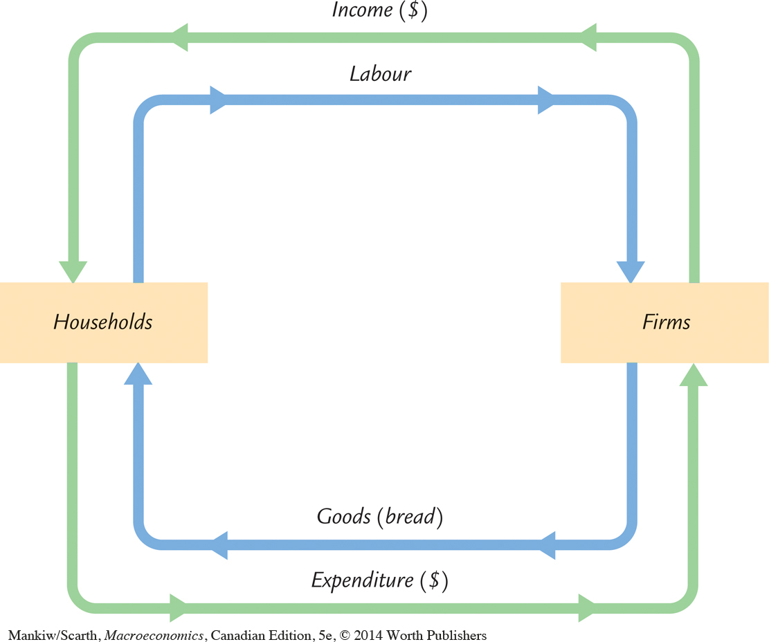
The outer loop in Figure 2-1 represents the corresponding flow of dollars. The households buy bread from the firms. The firms use some of the revenue from these sales to pay the wages of their workers, and the remainder is the profit belonging to the owners of the firms (who themselves are part of the household sector). Hence, expenditure on bread flows from households to firms, and income in the form of wages and profit flows from firms to households.
GDP measures the flow of dollars in this economy. We can compute it in two ways. GDP is the total income from the production of bread, which equals the sum of wages and profit—the top half of the circular flow of dollars. GDP is also the total expenditure on purchases of bread—the bottom half of the circular flow of dollars. To compute GDP, we can look at either the flow of dollars from firms to households or the flow of dollars from households to firms.
These two ways of computing GDP must be equal because the expenditure of buyers on products is, by the rules of accounting, income to the sellers of those products. Every transaction that affects expenditure must affect income, and every transaction that affects income must affect expenditure. For example, suppose that a firm produces and sells one more loaf of bread to a household. Clearly this transaction raises total expenditure on bread, but it also has an equal effect on total income. If the firm produces the extra loaf without hiring any more labour (such as by making the production process more efficient), then profit increases. If the firm produces the extra loaf by hiring more labour, then wages increase. In both cases, expenditure and income increase equally.
Some Rules for Computing GDP
22
In an economy that produces only bread, we can compute GDP by adding up the total expenditure on bread. Real economies, however, include the production and sale of a vast number of goods and services. To compute GDP for such a complex economy, it will be helpful to rely on the more precise definition given above: Gross domestic product (GDP) is the market value of all final goods and services produced within an economy in a given period of time. To see how this definition is applied, let’s discuss some of the rules that economists follow in constructing this statistic.
23
Adding Apples and Oranges The Canadian economy produces many different goods and services—hamburgers, haircuts, cars, computers, and so on. GDP combines the value of these goods and services into a single measure. The diversity of products in the economy complicates the calculation of GDP because different products have different values.
Suppose, for example, that the economy produces four apples and three oranges. How do we compute GDP? We could simply add apples and oranges and conclude that GDP equals seven pieces of fruit. But this makes sense only if we thought apples and oranges had equal value, which is generally not true. (This would be even clearer if the economy had produced four watermelons and three grapes.)
FYI
Stocks and Flows
Many economic variables measure a quantity of something—a quantity of money, a quantity of goods, and so on. Economists distinguish between two types of quantity variables: stocks and flows. A stock is a quantity measured at a given point in time, whereas a flow is a quantity measured per unit of time.
A bathtub, as shown in Figure 2-2, is the classic example used to illustrate stocks and flows. The amount of water in the tub is a stock: it is the quantity of water in the tub at a given point in time. The amount of water coming out of the faucet is a flow: it is the quantity of water being added to the tub per unit of time. Note that we measure stocks and flows in different units. We say that the bathtub contains 50 litres of water, but that water is coming out of the faucet at 5 litres per minute.
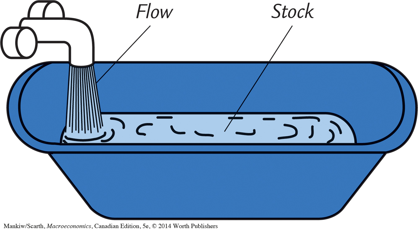
GDP is probably the most important flow variable in economics: it tells us how many dollars are flowing around the economy’s circular flow per unit of time. When you hear someone say that the Canadian GDP is $1.6 trillion, you should understand that this means that it is $1.6 trillion per year. (Equivalently, we could say that Canadian GDP is $4.38 billion per day.)
Stocks and flows are often related. In the bathtub example, these relationships are clear. The stock of water in the tub represents the accumulation of the flow out of the faucet, and the flow of water represents the change in the stock. When building theories to explain economic variables, it is often useful to determine whether the variables are stocks or flows and whether any relationships link them.
Here are some examples of related stocks and flows that we study in future chapters:
A person’s wealth is a stock; his income and expenditure are flows.
The number of unemployed people is a stock; the number of people losing their jobs is a flow.
The amount of capital in the economy is a stock; the amount of investment is a flow.
The government debt is a stock; the government budget deficit is a flow.
To compute the total value of different goods and services, the national accounts use market prices because these prices reflect how much people are willing to pay for a good or service. Thus, if apples cost $0.50 each and oranges cost $1.00 each, GDP would be
24
GDP = (Price of Apples × Quantity of Apples) + (Price of Oranges × Quantity of Oranges)
= ($0.50 × 4) + ($1.00 × 3)
= $5.00.
GDP equals $5.00—the value of all the apples, $2.00, plus the value of all the oranges, $3.00.
Used Goods When a sporting goods company makes a package of hockey cards and sells it for 50 cents, that 50 cents is added to the nation’s GDP. But what about when a collector sells a rare Rocket Richard card to another collector for $500? That $500 is not part of GDP. GDP measures the value of currently produced goods and services. The sale of the Rocket Richard card reflects the transfer of an asset, not an addition to the economy’s income. Thus, the sale of used goods is not included as part of GDP. Similarly, when an individual buys a financial asset, this transaction is not counted as part of the GDP. This is because a swap of one pre-existing asset (money) for another (the stock or bond) does not involve any productive activity. For this same reason, however, the financial services provider’s wages are counted in the GDP.
The Treatment of Inventories Imagine that a bakery hires workers to produce more bread, pays their wages, and then fails to sell the additional bread. How does this transaction affect GDP?
The answer depends on what happens to the unsold bread. Let’s first suppose that the bread spoils. In this case, the firm has paid more in wages but has not received any additional revenue, so the firm’s profit is reduced by the amount that wages have increased. Total expenditure in the economy hasn’t changed because no one buys the bread. Total income hasn’t changed either—although more is distributed as wages and less as profit. Because the transaction affects neither expenditure nor income, it does not alter GDP.
Now suppose, instead, that the bread is put into inventory to be sold later. In this case, the transaction is treated differently. The owners of the firm are assumed to have “purchased” the bread for the firm’s inventory, and the firm’s profit is not reduced by the additional wages it has paid. Because the higher wages raise total income, and greater spending on inventory raises total expenditure, the economy’s GDP rises.
What happens later when the firm sells the bread out of inventory? This case is much like the sale of a used good. There is spending by bread consumers, but there is inventory disinvestment by the firm. This negative spending by the firm offsets the positive spending by consumers, so the sale out of inventory does not affect GDP.
The general rule is that when a firm increases its inventory of goods, this investment in inventory is counted as expenditure by the firm owners. Thus, production for inventory increases GDP just as much as production for final sale. A sale out of inventory, however, is a combination of positive spending (the purchase) and negative spending (inventory disinvestment), so it does not influence GDP. This treatment of inventories ensures that GDP reflects the economy’s current production of goods and services.
25
Intermediate Goods and Value Added Many goods are produced in stages: raw materials are processed into intermediate goods by one firm and then sold to another firm for final processing. How should we treat such products when computing GDP? For example, suppose a cattle rancher sells one-quarter pound of meat to McDonald’s for $0.50, and then McDonald’s sells you a hamburger for $1.50. Should GDP include both the meat and the hamburger (a total of $2.00), or just the hamburger ($1.50)?
The answer is that GDP includes only the value of final goods. Thus, the hamburger is included in GDP but the meat is not: GDP increases by $1.50, not by $2.00. The reason is that the value of intermediate goods is already included as part of the market price of the final goods in which they are used. To add the intermediate goods to the final goods would be double counting—that is, the meat would be counted twice. Hence, GDP is the total value of final goods and services produced.
One way to compute the value of all final goods and services is to sum the value added at each stage of production. The value added of a firm equals the value of the firm’s output less the value of the intermediate goods that the firm purchases. In the case of the hamburger, the value added of the rancher is $0.50 (assuming that the rancher bought no intermediate goods), and the value added of McDonald’s is $1.50 − $0.50, or $1.00. Total value added is $0.50 + $1.00, which equals $1.50. For the economy as a whole, the sum of all value added must equal the value of all final goods and services. Hence, GDP is also the total value added of all firms in the economy.
Housing Services and Other Imputations Although most goods and services are valued at their market prices when computing GDP, some are not sold in the marketplace and therefore do not have market prices. If GDP is to include the value of these goods and services, we must use an estimate of their value. Such an estimate is called an imputed value.
Imputations are especially important for determining the value of housing. A person who rents a house is buying housing services and providing income for the landlord; the rent is part of GDP, both as expenditure by the renter and as income for the landlord. Many people, however, live in their own homes. Although they do not pay rent to a landlord, they are enjoying housing services similar to those that renters purchase. To take account of the housing services enjoyed by homeowners, GDP includes the “rent” that these homeowners “pay” to themselves. Of course, homeowners do not in fact pay themselves this rent. Statistics Canada estimates what the market rent for a house would be if it were rented and includes that imputed rent as part of GDP. This imputed rent is included both in the homeowner’s expenditure and in the homeowner’s income.
Imputations also arise in valuing government services. For example, police officers, fire fighters, and legislators provide services to the public. Giving a value to these services is difficult because they are not sold in a marketplace and therefore do not have a market price. The national accounts include these services in GDP by valuing them at their cost. That is, the wages of these public servants are used as a measure of the value of their output.
26
In many cases, an imputation is called for in principle but, to keep things simple, is not made in practice. Because GDP includes the imputed rent on owner-occupied houses, one might expect it also to include the imputed rent on cars, lawn mowers, jewellery, and other durable goods owned by households. Yet the value of these rental services is left out of GDP. In addition, some of the output of the economy is produced and consumed at home and never enters the marketplace. For example, meals cooked at home are similar to meals cooked at a restaurant, yet the value added in meals at home is left out of GDP. Statistics Canada does not try to estimate the value of “household production” like this on any regular basis. Just to give some idea of the magnitude involved, however, the agency published an estimate for 1991. According to this study, household production in Canada is equal to about one-third of the measured GDP.
Finally, no imputation is made for the value of goods and services sold in the underground economy. The underground economy is the part of the economy that people hide from the government either because they wish to evade taxation or because the activity is illegal. Home construction, repairs, and cleaning services paid “under the table” are examples of the underground economy. The illegal drug trade is another.
Because the imputations necessary for computing GDP are only approximate, and because the value of many goods and services is left out altogether, GDP is an imperfect measure of total economic activity. These imperfections are most problematic when comparing standards of living across countries. The size of the underground economy, for instance, varies from country to country. Yet as long as the magnitude of these imperfections remains fairly constant over time, GDP is useful for comparing economic activity from year to year.
Real GDP versus Nominal GDP
Economists use the rules just described to compute GDP, which values the economy’s total output of goods and services. But is GDP a good measure of economic well-being? Consider once again the economy that produces only apples and oranges. In this economy GDP is the sum of the value of all the apples produced and the value of all the oranges produced. That is,
GDP = (Price of Apples × Quantity of Apples) + (Price of Oranges × Quantity of Oranges).
Economists call the value of goods and services measured at current prices nominal GDP. Notice that nominal GDP can increase either because prices rise or because quantities rise.
It is easy to see that GDP computed this way is not a good gauge of economic well-being. That is, this measure does not accurately reflect how well the economy can satisfy the demands of households, firms, and the government. If all prices doubled without any change in quantities, GDP would double. Yet it would be misleading to say that the economy’s ability to satisfy demands has doubled, because the quantity of every good produced remains the same.
A better measure of economic well-being would tally the economy’s output of goods and services without being influenced by changes in prices. For this purpose, economists use real GDP, which is the value of goods and services measured using a constant set of prices. That is, real GDP shows what would have happened to expenditure on output if quantities had changed but prices had not.
27
To see how real GDP is computed, imagine we wanted to compare output in 2009, 2010, and 2011 in our apple-and-orange economy. We could begin by choosing a set of prices, called base-year prices, such as the prices that prevailed in 2009. Goods and services are then added up using these base-year prices to value the different goods in both years. Real GDP for 2009 would be
Real GDP = (2009 Price of Apples × 2009 Quantity of Apples) + (2009 Price of Oranges × 2009 Quantity of Oranges).
Similarly, real GDP in 2010 would be
Real GDP = (2009 Price of Apples × 2010 Quantity of Apples) + (2009 Price of Oranges × 2010 Quantity of Oranges).
And real GDP in 2011 would be
Real GDP = (2009 Price of Apples × 2011 Quantity of Apples) + (2009 Price of Oranges × 2011 Quantity of Oranges).
Notice that 2009 prices are used to compute real GDP for all three years. Because the prices are held constant, real GDP varies from year to year only if the quantities produced vary. Because a society’s ability to provide economic satisfaction for its members ultimately depends on the quantities of goods and services produced, real GDP provides a better measure of economic well-being than nominal GDP.
The GDP Deflator
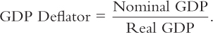
From nominal GDP and real GDP we can compute a third statistic: the GDP deflator. The GDP deflator, also called the implicit price deflator for GDP, is defined as the ratio of nominal GDP to real GDP:
The GDP deflator reflects what’s happening to the overall level of prices in the economy.
To understand this better, consider again an economy with only one good, bread. If P is the price of bread and Q is the quantity sold, then nominal GDP is the total number of dollars spent on bread in that year, P × Q. Real GDP is the number of loaves of bread produced in that year times the price of bread in some base year, Pbase × Q. The GDP deflator is the price of bread in that year relative to the price of bread in the base year, P/Pbase.
The definition of the GDP deflator allows us to separate nominal GDP into two parts: one part measures quantities (real GDP) and the other measures prices (the GDP deflator). That is,
28
Nominal GDP = Real GDP × GDP Deflator.
Nominal GDP measures the current dollar value of the output of the economy. Real GDP measures output valued at constant prices. The GDP deflator measures the price of output relative to its price in the base year.
We can also write this equation as
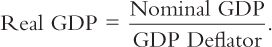
In this form, you can see how the deflator earns its name: it is used to deflate (that is, take inflation out of) nominal GDP to yield real GDP.
Chain-Weighted Measures of Real GDP
We have been discussing real GDP as if the prices used to compute this measure never change from their base-year values. If this were truly the case, over time the prices would become more and more dated. For instance, the price of computers has fallen substantially in recent years, while the price of a year at university has risen. When valuing the production of computers and education, it would be misleading to use the prices that prevailed ten or twenty years ago.
To solve this problem, the traditional approach involved Statistics Canada updating periodically the prices used to compute real GDP. About every five years, a new base year was chosen. The prices were then held fixed and used to measure year-to-year changes in the production of goods and services until the base year is updated once again.
Since 2001 Statistics Canada has been using a new policy for dealing with changes in the base year. In particular, it now calculates chain-weighted measures of real GDP. With these new measures, the base year changes continuously over time. In essence, average prices in 2008 and 2009 are used to measure real growth from 2008 to 2009; average prices in 2009 and 2010 are used to measure real growth from 2009 to 2010; and so on. These various year-to-year growth rates are then put together to form a “chain” that can be used to compare the output of goods and services between any two dates.
This new chain-weighted measure of real GDP is better than the more traditional measure because it ensures that the prices used to compute real GDP are never far out of date. For most purposes, however, the differences are not significant. It turns out that the two measures of real GDP are highly correlated with each other. As a practical matter, then, both the old and new measures of real GDP reflect the same thing: economy-wide changes in the production of goods and services.
The Components of Expenditure
Economists and policymakers care not only about the economy’s total output of goods and services but also about the allocation of this output among alternative uses. The national accounts divide GDP into four broad categories of spending:
Consumption (C)
Investment (I)
29
Government purchases (G)
Net exports (NX).
Thus, letting Y stand for GDP,
Y = C + I + G + NX.
GDP is the sum of consumption, investment, government purchases, and net exports. Each dollar of GDP falls into one of these categories. This equation is an identity—an equation that must hold because of the way the variables are defined. It is called the national accounts identity.
Consumption consists of the goods and services bought by households. It is divided into three subcategories: durable goods, nondurable goods, and services. Durable goods are goods that last a long time, such as cars and TVs. Nondurable goods are goods that last only a short time, such as food and clothing. Services include the work done for consumers by individuals and firms, such as haircuts and doctor visits.
FYI
Two Arithmetic Tricks for Working With Percentage Changes
For manipulating many relationships in economics, there is an arithmetic trick that is useful to know: The percentage change of a product of two variables is approximately the sum of the percentage changes in each of the variables.
To see how this trick works, consider an example. Let P denote the GDP deflator and Y denote real GDP. Nominal GDP is P × Y. The trick states that
Percentage Change in (P × Y) ≈ (Percentage Change in P) + (Percentage Change in Y).
For instance, suppose that in one year, real GDP is 100 and the GDP deflator is 2; the next year, real GDP is 103 and the GDP deflator is 2.1. We can calculate that real GDP rose by 3 percent and that the GDP deflator rose by 5 percent. Nominal GDP rose from 200 the first year to 216.3 the second year, an increase of 8.15 percent. Notice that the growth in nominal GDP (8.15 percent) is approximately the sum of the growth in the GDP deflator (5 percent) and the growth in real GDP (3 percent).1
A second arithmetic trick follows as a corollary to the first: The percentage change of a ratio is approximately the percentage change in the numerator minus the percentage change in the denominator. Again, consider an example. Let Y denote GDP and L denote the population, so that Y/L is GDP per person. The second trick states
Percentage Change in (Y/L) ≈ (Percentage Change in Y ) – (Percentage Change in L).
For instance, suppose that in the first year, Y is 100,000 and L is 100, so Y/L is 1,000; in the second year, Y is 110,000 and L is 103, so Y/L is 1,068. Notice that the growth in GDP per person (6.8 percent) is approximately the growth in income (10 percent) minus the growth in population (3 percent).
30
FYI
What Is Investment?
Newcomers to macroeconomics are sometimes confused by how macroeconomists use familiar words in new and specific ways. One example is the term “investment.” The confusion arises because what looks like investment for an individual may not be investment for the economy as a whole. The general rule is that the economy’s investment does not include purchases that merely reallocate existing assets among different individuals. Investment, as macroeconomists use the term, creates new capital.
Let’s consider some examples. Suppose we observe these two events:
Smith buys for himself a 100-year-old Victorian house.
Jones builds for herself a brand-new contemporary house.
What is total investment here? Two houses, one house, or zero?
A macroeconomist seeing these two transactions counts only the Jones house as investment. Smith’s transaction has not created new housing for the economy; it has merely reallocated existing housing. Smith’s purchase is investment for Smith, but it is disinvestment for the person selling the house. By contrast, Jones has added new housing to the economy; her new house is counted as investment.
Similarly, consider these two events:
Clarke buys $5 million in Air Canada stock from White on the Toronto Stock Exchange.
Toyota sells $10 million in stock to the public and uses the proceeds to build a new car factory.
Here, investment is $10 million. In the first transaction, Clarke is investing in Air Canada stock, and White is disinvesting; there is no investment for the economy. By contrast, Toyota is using some of the economy’s output of goods and services to add to its stock of capital; hence, its new factory is counted as investment.
Finally, consider this event:
Black buys $2 million of Toyota stock.
This transaction simply involves Black swapping one financial asset for another. While such transactions are referred to as investments in the financial press, this transaction is not an investment in terms of how economists use this term.
Investment consists of goods bought for future use. Investment is also divided into three subcategories: business fixed investment, residential construction, and inventory investment. Business fixed investment is the purchase of a new plant and equipment by firms. Residential construction is the purchase of new housing by households and landlords. Inventory investment is the increase in firms’ inventories of goods (if inventories are falling, inventory investment is negative).
Government purchases are the goods and services bought by federal, provincial, and municipal governments. This category includes such items as military equipment, highways, and the services that government workers provide. It does not include transfer payments to individuals, such as the Canada Pension, employment insurance benefits, and welfare. Because transfer payments reallocate existing income and are not made in exchange for currently produced goods and services, they are not part of GDP.
31
The last category, net exports, accounts for trade with other countries. Net exports are the value of goods and services sold to other countries (our exports) minus the value of goods and services that foreigners sell us (our imports). Net exports are positive when the value of our exports is greater than the value of our imports and negative when the value of our imports is greater than the value of our exports. Net exports represent the net expenditure from abroad on our goods and services, which provides income for domestic producers.
CASE STUDY
GDP and Its Components
In 2012 the GDP of Canada totaled 1658 billion. This number is so large that it is almost impossible to comprehend. We can make it easier to understand by dividing it by the 2012 Canadian population of 34.88 million. In this way, we obtain GDP per person—the amount of expenditure for the average Canadian—which equaled $47,533 in 2012.
How did we use this GDP? Table 2-1 shows that just under 56 percent of it, or $26,461 per person, was spent on consumption. Investment was $11,267 per person, and government purchases were $11,905 per person (so government programs represented about 23 percent of the economy).
| Total (billions of dollars) | Per Person (dollars) | |
| Gross Domestic Product | $1,658 | $47,533 |
| Consumption | 923 | 26,461 |
| Durables and nondurables | 424 | 12,155 |
| Services | 499 | 14,305 |
| Investment | 393 | 11,267 |
| Business fixed investment (factories, machinery) | 276 | 7,912 |
| Residential construction | 112 | 3,210 |
| Inventory investment | 5 | 143 |
| Government Purchases | 387 | 11,095 |
| Net Exports | –45 | –1,290 |
| Exports | 506 | 14,506 |
| Imports | 551 | 15,796 |
|
Source: Statistics Canada, National Income and Expenditure Accounts, http://www.statcan.gc.ca/pub/13-010-x/2009001/t/tab03-eng.htm |
||
|---|---|---|
32
The average person bought $15,796 of goods imported from abroad and produced $14,506 of goods that were exported to other countries. Thus, net exports were a small negative amount. Since we earned less from selling to foreigners than we spent on foreign goods, we covered the difference by increasing slightly the country’s foreign debt.
It is interesting to compare how Canadians use their GDP to the spending patterns in other countries. Even when compared to Americans, there are significant differences. While Canadians spend 33.2 percent of per-capita GDP on imports, Americans limit spending on imports to 17 percent. Canadians leave 23.3 percent of per-capita GDP to be spent by various levels of government, while Americans limit this proportion to 19 percent. 
Several Measures of Income
The national accounts include other measures of income that differ slightly in definition from GDP. It is important to be aware of the various measures, because economists and the press often refer to them.
We can see how the alternative measures of income relate to one another, by starting with GDP and subtracting various quantities. As explained above, to obtain the gross total of Canadian income that flows from GDP, the GNP, we subtract the net income of foreigners who own factors of production employed in Canada:
Gross National Income = GDP – Net Income of Foreigners.
To obtain net national income, we subtract the depreciation of capital—the amount of the economy’s stock of plants, equipment, and residential structures that wears out during the year:
Net National Income = Gross National Income – Depreciation.
In the national accounts, depreciation is called the capital consumption allowances. In 2012, it equaled about 16 percent of gross national income. Since the depreciation of capital is a cost of producing the output of the economy, subtracting depreciation shows the net result of economic activity. For this reason, some economists believe that net national income is a better measure of economic well-being.
The next adjustment in the national accounts is for indirect business taxes, such as sales taxes. These taxes, which make up 12 percent of net national income, place a wedge between the price that consumers pay for a good and the price that firms receive. Because firms never receive this tax wedge, it is not part of their income. Once we subtract indirect business taxes, we obtain a measure called simply national income. National income is a measure of how much everyone in the economy has earned.
33
The national accounts divide national income into three components, depending on the way the income is earned. The three categories, and the percentage of national income that each comprises, in 2012, are:
Compensation of employees (68.5 percent). The wages and fringe benefits earned by workers
Corporate profits (19.5 percent). The income of corporations after payments to their workers and creditors
Nonincorporated business and net interest income (12 percent). The income of noncorporate businesses, such as small farms and law partnerships, and the income that landlords receive, including the imputed rent that homeowners “pay” to themselves, less expenses, such as depreciation; and the interest domestic businesses pay minus the interest they receive, plus interest earned from foreigners.
A series of adjustments takes us from national income to personal income, the amount of income that households and noncorporate businesses receive. Three of these adjustments are most important. First, we reduce national income by the amount that corporations earn but do not pay out, either because the corporations are retaining earnings or because they are paying taxes to the government. This adjustment is made by subtracting corporate profits (which equals the sum of corporate taxes, dividends, and retained earnings) and adding back dividends. Second, we increase national income by the net amount the government pays out in transfer payments. This adjustment equals government transfers to individuals minus social insurance contributions paid to the government. Third, we adjust national income to include the interest that households earn rather than the interest that businesses pay. This adjustment is made by adding personal interest income and subtracting net interest. (The difference between personal interest and net interest arises in part from the interest on the government debt.) Thus, personal income is
Personal Income = National Income
– Corporate Profits
– Social Insurance Contributions
– Net Interest
+ Dividends
+ Government Transfers to Individuals
+ Personal Interest Income.
Next, if we subtract personal tax payments, we obtain personal disposable income:
Personal Disposable Income = Personal Income – Personal Tax Payments.
We are interested in personal disposable income because it is the amount households and noncorporate businesses have available to spend after satisfying their tax obligations to the government.
34
CASE STUDY
Seasonal Adjustment
Because real GDP and the other measures of income reflect how well the economy is performing, economists are interested in studying the quarter-to-quarter fluctuations in these variables. Yet when we start to do so, one fact leaps out: all these measures of income exhibit a regular seasonal pattern. The output of the economy rises during the year, reaching a peak in the fourth quarter (October, November, and December), and then falling in the first quarter (January, February, and March) of the next year. These regular seasonal changes are substantial. From the fourth quarter to the first quarter, real GDP falls on average about 5 percent.2
It is not surprising that real GDP follows a seasonal cycle. Some of these changes are attributable to changes in our ability to produce: for example, building homes is more difficult during the cold weather of winter than during other seasons. In addition, people have seasonal tastes: they have preferred times for such activities as vacations and Christmas shopping.
When economists study fluctuations in real GDP and other economic variables, they often want to eliminate the portion of fluctuations due to predictable seasonal changes. You will find that most of the economic statistics reported in the newspaper are seasonally adjusted. This means that the data have been adjusted to remove the regular seasonal fluctuations. Therefore, when you observe a rise or fall in real GDP or any other data series, you must look beyond the seasonal cycle for the explanation.