3.2 How Is National Income Distributed to
the Factors of Production?
53
As we discussed in Chapter 2, the total output of an economy equals its total income. Because the factors of production and the production function together determine the total output of goods and services, they also determine national income. The circular flow diagram in Figure 3-1 shows that this national income flows from firms to households through the markets for the factors of production.
In this section we continue to develop our model of the economy by discussing how these factor markets work. Economists have long studied factor markets to understand the distribution of income. (For example, Karl Marx, the noted nineteenth-century economist, spent much time trying to explain the incomes of capital and labour. The political philosophy of communism was in part based on Marx’s now-discredited theory.)
Here we examine the modern theory of how national income is divided among the factors of production. It is based on the classical (18th century) idea that prices adjust to balance supply and demand (applied here to the markets for the factors of production) together with the more recent (19th century) idea that the demand for each factor of production depends on the marginal productivity of that factor. This theory, called the neoclassical theory of distribution, is accepted by most economists today as the best place to start in understanding how the economy’s income is distributed from firms to households.
Factor Prices
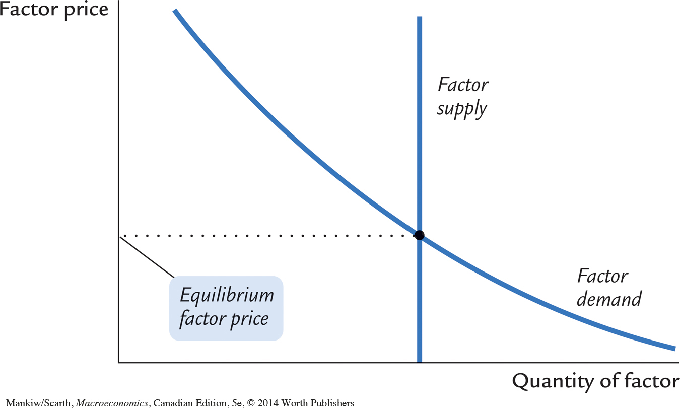
The distribution of national income is determined by factor prices. Factor prices are the amounts paid to the factors of production—the wage workers earn and the rent the owners of capital collect. As Figure 3-2 illustrates, the rental price each factor of production receives for its services is in turn determined by the supply and demand for that factor. Because we have assumed that the economy’s factors of production are fixed, the factor supply curve in Figure 3-2 is vertical. Regardless of the factor price, the quantity of the factor supplied to the market is the same. The intersection of the downward-sloping factor demand curve and the vertical supply curve determines the equilibrium factor price.
54
To understand factor prices and the distribution of income, we must examine the demand for the factors of production. Because factor demand arises from the thousands of firms that use capital and labour, we start by examining the decisions a typical firm makes about how much of these factors to employ.
The Decisions Facing the Competitive Firm
The simplest assumption to make about a typical firm is that it is competitive. A competitive firm is small relative to the markets in which it trades, so it has little influence on market prices. For example, our firm produces a good and sells it at the market price. Because many firms produce this good, our firm can sell as much as it wants without causing the price of the good to fall, or it can stop selling altogether without causing the price of the good to rise. Similarly, our firm cannot influence the wages of the workers it employs because many other local firms also employ workers. The firm has no reason to pay more than the market wage, and if it tried to pay less, its workers would take jobs elsewhere. Therefore, the competitive firm takes the prices of its output and its inputs as given by market conditions.
To make its product, the firm needs two factors of production, capital and labour. As we did for the aggregate economy, we represent the firm’s production technology by the production function
Y = F(K, L),
where Y is the number of units produced (the firm’s output), K the number of machines used (the amount of capital), and L the number of hours worked by the firm’s employees (the amount of labour). Holding constant the technology as expressed in the production function, the firm produces more output if it uses more machines or if its employees work more hours.
The firm sells its output at a price P, hires workers at a wage W, and rents capital at a rate R. Notice that when we speak of firms renting capital, we are assuming that households own the economy’s stock of capital. In this analysis, households rent out their capital, just as they sell their labour. The firm obtains both factors of production from the households that own them.1
55
The goal of the firm is to maximize profit. Profit is revenue minus costs—it is what the owners of the firm keep after paying for the costs of production. Revenue equals P × Y, the selling price of the good P multiplied by the amount of the good the firm produces Y. Costs include both labour costs and capital costs. Labour costs equal W × L, the wage W times the amount of labour L. Capital costs equal R × K, the rental price of capital R times the amount of capital K. We can write
Profit = Revenue – Labour Costs – Capital Costs
=PY–WL–RK.
To see how profit depends on the factors of production, we use the production function Y = F(K, L) to substitute for Y to obtain
Profit = PF(K, L) – WL – RK.
This equation shows that profit depends on the product price P, the factor prices W and R, and the factor quantities L and K. The competitive firm takes the product price and the factor prices as given and chooses the amounts of labour and capital that maximize profit.
The Firm’s Demand for Factors
We now know that our firm will hire labour and rent capital in the quantities that maximize profit. But how does it figure out what those profit-maximizing quantities are? To answer this question, we first consider the quantity of labour and then the quantity of capital.
The Marginal Product of Labour The more labour the firm employs, the more output it produces. The marginal product of labour (MPL) is the extra amount of output the firm gets from one extra unit of labour, holding the amount of capital fixed. We can express this using the production function:
MPL = F(K, L + 1) – F(K, L).
The first term on the right-hand side is the amount of output produced with K units of capital and L + 1 units of labour; the second term is the amount of output produced with K units of capital and L units of labour. This equation states that the marginal product of labour is the difference between the amount of output produced with L + 1 units of labour and the amount produced with only L units of labour.
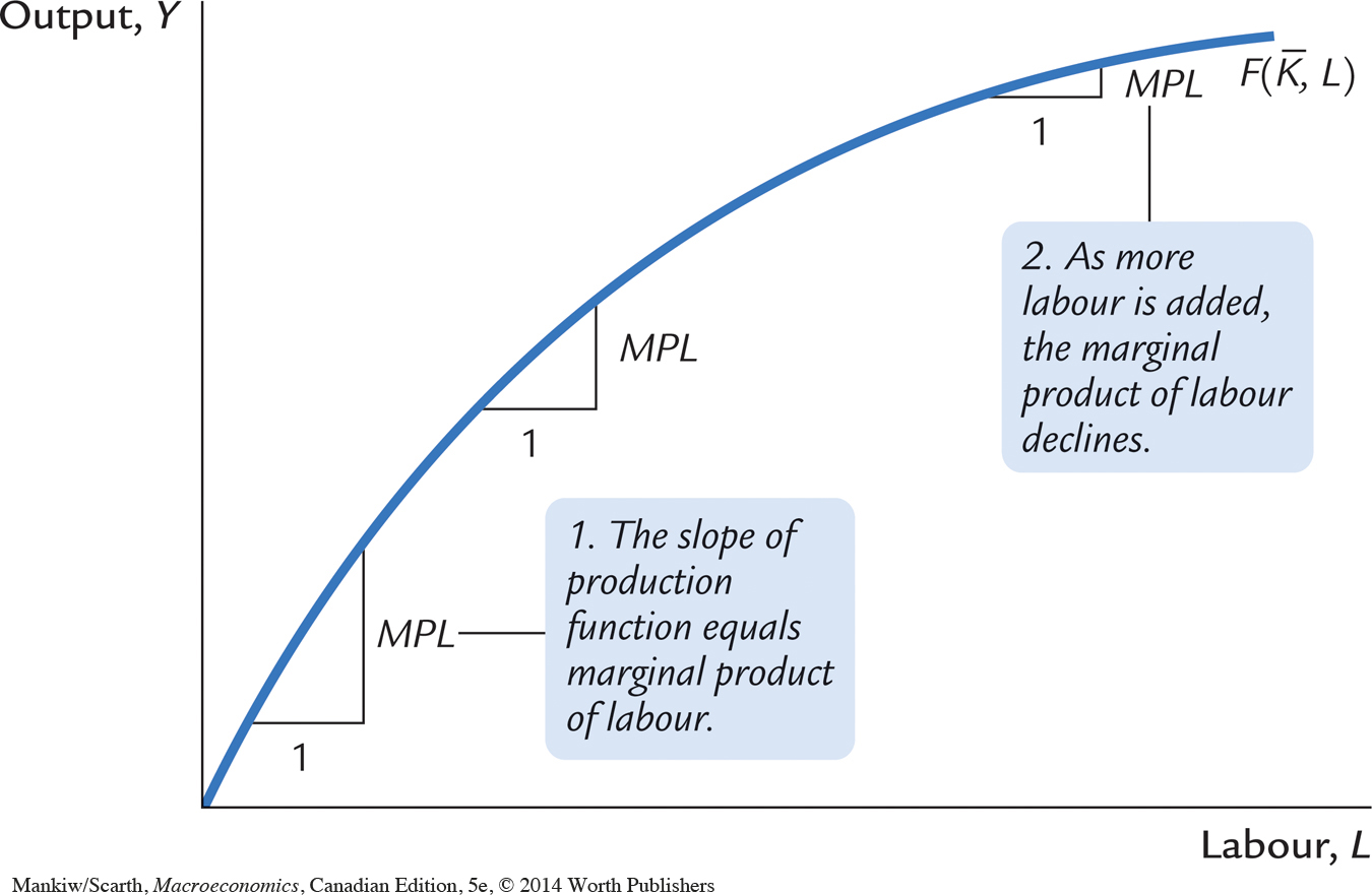
Most production functions have the property of diminishing marginal product: holding the amount of capital fixed, the marginal product of labour decreases as the amount of labour increases. To see why, consider again the production of bread at a bakery. As a bakery hires more labour, it produces more bread. The MPL is the amount of extra bread produced when an extra unit of labour is hired. As more labour is added to a fixed amount of capital, however, the MPL falls. Fewer additional loaves are produced because workers are less productive when the kitchen is more crowded. In other words, holding the size of the kitchen fixed, each additional worker adds fewer loaves of bread to the bakery’s output.
56
Figure 3-3 graphs the production function. It illustrates what happens to the amount of output when we hold the amount of capital constant and vary the amount of labour. This figure shows that the marginal product of labour is the slope of the production function. As the amount of labour increases, the production function becomes flatter, indicating diminishing marginal product.
From the Marginal Product of Labour to Labour Demand When the competitive, profit-maximizing firm is deciding whether to hire an additional unit of labour, it considers how that decision would affect profits. It therefore compares the extra revenue from the increased production that results from the added labour to the extra cost of higher spending on wages. The increase in revenue from an additional unit of labour depends on two variables: the marginal product of labour and the price of the output. Because an extra unit of labour produces MPL units of output and each unit of output sells for P dollars, the extra revenue is P × MPL. The extra cost of hiring one more unit of labour is the wage W. Thus, the change in profit from hiring an additional unit of labour is
ΔProfit = ΔRevenue – ΔCost
= (P × MPL) – W.
The symbol Δ (called delta) denotes the change in a variable.
57
We can now answer the question we asked at the beginning of this section: How much labour does the firm hire? The firm’s manager knows that if the extra revenue P × MPL exceeds the wage W, an extra unit of labour increases profit. Therefore, the manager continues to hire labour until the next unit would no longer be profitable—that is, until the MPL falls to the point where the extra revenue equals the wage. The competitive firm’s demand for labour is determined by
P × MPL = W.
We can also write this as
MPL = W/P.
W/P is the real wage—the payment to labour measured in units of output rather than in dollars. To maximize profit, the firm hires up to the point at which the marginal product of labour equals the real wage.
For example, again consider a bakery. Suppose the price of bread P is $2 per loaf, and a worker earns a wage W of $20 per hour. The real wage W/P is 10 loaves per hour. In this example, the firm keeps hiring workers as long as the additional worker would produce at least 10 loaves per hour. When the MPL falls to 10 loaves per hour or less, hiring additional workers is no longer profitable.
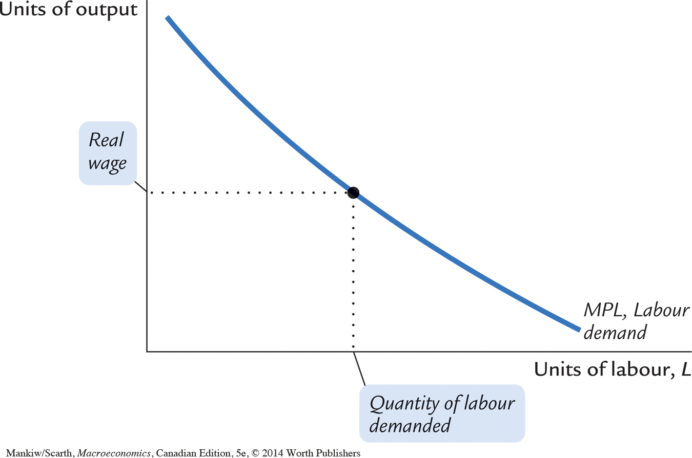
Figure 3-4 shows how the marginal product of labour depends on the amount of labour employed (holding the firm’s capital stock constant). That is, this figure graphs the MPL schedule. Because the MPL diminishes as the amount of labour increases, this curve slopes downward. For any given real wage, the firm hires up to the point at which the MPL equals the real wage. Hence, the MPL schedule is also the firm’s labour demand curve.
58
The Marginal Product of Capital and Capital Demand The firm decides how much capital to rent in the same way it decides how much labour to hire. The marginal product of capital (MPK) is the amount of extra output the firm gets from an extra unit of capital, holding the amount of labour constant:
MPK = F(K + 1, L) – F(K, L).
Thus, the marginal product of capital is the difference between the amount of output produced with K + 1 units of capital and that produced with only K units of capital.
Like labour, capital is subject to diminishing marginal product. Once again consider the production of bread at a bakery. The first several ovens installed in the kitchen will be very productive. However, if the bakery installs more and more ovens, while holding its labour force constant, it will eventually contain more ovens than its employees can effectively operate. Hence, the marginal product of the last few ovens is lower than that of the first few.
The increase in profit from renting an additional machine is the extra revenue from selling the output of that machine minus the machine’s rental price:
ΔProfit = ΔRevenue – ΔCost
= (P × MPK) – R.
To maximize profit, the firm continues to rent more capital until the MPK falls to equal the real rental price:
MPK = R/P.
The real rental price of capital is the rental price measured in units of goods rather than in dollars.
To sum up, the competitive, profit-maximizing firm follows a simple rule about how much labour to hire and how much capital to rent. The firm demands each factor of production until that factor’s marginal product falls to equal its real factor price.
The Division of National Income
Having analyzed how a firm decides how much of each factor to employ, we can now explain how the markets for the factors of production distribute the economy’s total income. If all firms in the economy are competitive and profit-maximizing, then each factor of production is paid its marginal contribution to the production process. The real wage paid to each worker equals the MPL, and the real rental price paid to each owner of capital equals the MPK. The total real wages paid to labour are therefore MPL × L, and the total real return paid to capital owners is MPK × K.
The income that remains after the firms have paid the factors of production is the economic profit of the owners of the firms. Real economic profit is
Economic Profit = Y – (MPL × L) – (MPK × K).
59
Because we want to examine the distribution of national income, we rearrange the terms as follows:
Y = (MPL × L) + (MPK × K) + Economic Profit.
Total income is divided among the return to labour, the return to capital, and economic profit.
How large is economic profit? The answer is surprising: if the production function has the property of constant returns to scale, as is often thought to be the case, then economic profit must be zero. That is, nothing is left after the factors of production are paid. This conclusion follows from a famous mathematical result called Euler’s theorem,2 which states that if the production function has constant returns to scale, then
F(K, L) = (MPK × K) + (MPL × L).
If each factor of production is paid its marginal product, then the sum of these factor payments equals total output. In other words, constant returns to scale, profit maximization, and competition together imply that economic profit is zero.
If economic profit is zero, how can we explain the existence of “profit” in the economy? The answer is that the term “profit” as normally used is different from economic profit. We have been assuming that there are three types of agents: workers, owners of capital, and owners of firms. Total income is divided among wages, return to capital, and economic profit. In the real world, however, most firms own rather than rent the capital they use. Because firm owners and capital owners are the same people, economic profit and the return to capital are often lumped together. If we call this alternative definition accounting profit, we can say that
Accounting Profit = Economic Profit + (MPK × K).
Under our assumptions—constant returns to scale, profit maximization, and competition—economic profit is zero. If these assumptions approximately describe the world, then the “profit” in the national income accounts must be mostly the return to capital.
We can now answer the question posed at the beginning of this chapter about how the income of the economy is distributed from firms to households. Each factor of production is paid its marginal product, and these factor payments exhaust total output. Total output is divided between the payments to capital and the payments to labour, depending on their marginal productivities.
60
CASE STUDY
The Black Death and Factor Prices
According to the neoclassical theory of distribution, factor prices equal the marginal products of the factors of production. Because the marginal products depend on the quantities of the factors, a change in the quantity of any one factor alters the marginal products of all the factors. Therefore, a change in the supply of a factor alters equilibrium factor prices.
Fourteenth-century Europe provides a vivid example of how factor quantities affect factor prices. The outbreak of the bubonic plague—the Black Death—in 1348 reduced the population of Europe by about one-third within a few years. Because the marginal product of labour increases as the amount of labour falls, this massive reduction in the labour force raised the marginal product of labour. (The economy moved to the left along the curves in Figures 3-3 and 3-4.) Real wages did increase substantially during the plague years—doubling, by some estimates. The peasants who were fortunate enough to survive the plague enjoyed economic prosperity.
The reduction in the labour force caused by the plague also affected the return to land, the other major factor of production in medieval Europe. With fewer workers available to farm the land, an additional unit of land produced less additional output. This fall in the marginal product of land led to a decline in real rents of 50 percent or more. Thus, while the peasant classes prospered, the landed classes suffered reduced incomes.3 
The Cobb–Douglas Production Function
What production function describes how actual economies turn capital and labour into GDP? The answer to this question came from a historic collaboration between a U.S. senator and a mathematician.
Paul Douglas was a U.S. senator from Illinois from 1949 to 1966. In 1927, however, when he was still a professor of economics, he noticed a surprising fact: the division of national income between capital and labour had been roughly constant over a long period. In other words, as the economy grew more prosperous over time, the total income of workers and the total income of capital owners grew at almost exactly the same rate. This observation caused Douglas to wonder what conditions lead to constant factor shares.
Douglas asked Charles Cobb, a mathematician, what production function, if any, would produce constant factor shares if factors always earned their marginal products. The production function would need to have the property that
Capital Income = MPK × K = αY,
and
Labour Income = MPL × L = (1 – α) Y,
61
where α is a constant between zero and one that measures capital’s share of income. That is, α determines what share of income goes to capital and what share goes to labour. Cobb showed that the function with this property is
Y = F(K,L) = A K αL1 – α,
where A is a parameter greater than zero that measures the productivity of the available technology. This function became known as the Cobb–Douglas production function.
Let’s take a closer look at some of the properties of this production function. First, the Cobb–Douglas production function has constant returns to scale. That is, if capital and labour are increased by the same proportion, then output increases by that proportion as well.4
Next, consider the marginal products for the Cobb–Douglas production function. The marginal product of labour is5
MPL = (1 – α) AKαL–α
and the marginal product of capital is
MPK = αAKα–1L1–α.
From these equations, recalling that α is between zero and one, we can see what causes the marginal products of the two factors to change. An increase in the amount of capital raises the MPL and reduces the MPK. Similarly, an increase in the amount of labour reduces the MPL and raises the MPK. A technological advance that increases the parameter A raises the marginal product of both factors proportionately.
The marginal products for the Cobb–Douglas production function can also be written as6
62
MPL = (1 – α)Y/L.
MPK = αY/K.
The MPL is proportional to output per worker, and the MPK is proportional to output per unit of capital. Y/L is called average labour productivity, and Y/K is called average capital productivity. If the production function is Cobb–Douglas, then the marginal productivity of a factor is proportional to its average productivity.
We can now verify that if factors earn their marginal products, then the parameter α indeed tells us how much income goes to labour and how much goes to capital. The total wage bill, which we have seen is MPL × L, equals (1 – α)Y. Therefore, (1 – α) is labour’s share of output. Similarly, the total return to capital, MPK × K, is αY, and α is capital’s share of output. The ratio of labour income to capital income is a constant, (1 – α)/α, just as Douglas observed. The factor shares depend only on the parameter α, not on the amounts of capital or labour or on the state of technology as measured by the parameter A.
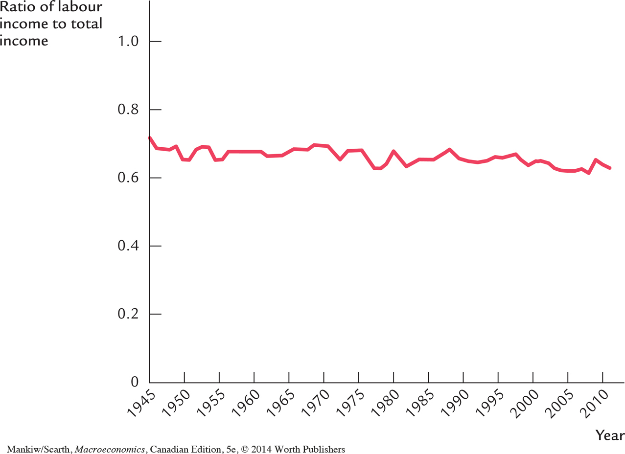
More recent data are also consistent with the Cobb–Douglas production function. Figure 3-5 shows the ratio of labour income to total income in Canada from 1945 to 2010. Despite the many changes in the economy over 65 years, this ratio has remained just under two-thirds. This division of income is easily explained by a Cobb–Douglas production function in which the parameter α is about 0.33. According to this parameter, capital receives one-third of income, and labour receives two-thirds.
The Cobb-Douglas production function is not the last word in explaining the economy’s production of goods and services or the distribution of national income between capital and labour. It is, however, a good place to start.
CASE STUDY
Labour Productivity as the Key Determinant of Real Wages
The neoclassical theory of distribution tells us that the real wage W/P equals the marginal product of labour. The Cobb-Douglas production function tells us that the marginal product of labour is proportional to average labour productivity Y/L. If this theory is right, then workers should enjoy rapidly rising living standards when labour productivity is growing robustly. Is this true?
Table 3-1 presents some data on growth in productivity and real wages for the Canadian economy, over a 46-year period. From 1961 to 2007, productivity as measured by output per unit of labour input grew at 1.7 percent per year. Real wages grew at the same rate of 1.7 percent. With a growth rate such as this, productivity and real wages double about every 42 years.
| Time Period | Labour Productivity Growth | Real Wage Growth |
| 1961–2007 | 1.7% | 1.7% |
| 1961–1973 | 3.0% | 3.9% |
| 1973–1981 | 1.3% | 1.4% |
| 1981–1989 | 1.2% | 0.3% |
| 1989–2000 | 1.5% | 0.8% |
| 2000–2007 | 1.0% | 1.2% |
|
Source: www.csls.ca/ipm/17/IPM-17-sharpe.pdf |
||
|---|---|---|
63
Productivity growth varies over time. The table shows the data for four shorter periods that economists have identified as having different productivity experiences. (Case Studies in Chapter 8 examine some of the reasons for these changes in productivity growth.) Around 1973, both the Canadian and U.S. economies experienced a significant slowdown in productivity growth. The cause of the productivity slowdown is not well understood, but the link between productivity and real wages is exactly as standard theory predicts. The slowdown in productivity growth from 3.0% in the earlier period (1961–1973) to 1.3% in the 1973–1981 period coincided with a slowdown in real wage growth from 3.9 to 1.4 percent per year. A similar correspondence between productivity growth and real wage growth is evident in the more recent sub-periods in Table 3-1.
There are two disturbing features about recent developments in Canada. The first involves comparing our productivity performance with that in the United States. In the United States, productivity growth picked up again around 1995, and many observers hailed the arrival of the “new economy.” This productivity acceleration is often attributed to the spread of computers and information technology. As theory predicts, growth in real wages picked up as well—but only in the United States. As we can see in the table, there has not been the same rebound in productivity growth (and, therefore, in real wage growth) in Canada. The resulting growing gap between material living standards in the United States and Canada has many Canadian policymakers concerned.
64
The second issue that has puzzled analysts somewhat is that since 1981, real wage growth has lagged behind productivity growth to some extent. Contrary to Canada’s earlier experience, labour productivity growth has exceeded real wage growth by an accumulated amount equal to 37 percent over this 26-year period. You can learn the reasons by reading an article written by Sharpe, Arsenault, and Harrison entitled “Why Have Real Wages Lagged Productivity Growth in Canada?” It was published in the Fall 2008 issue of the International Productivity Monitor and is available on the website given as the source for Table 3-1.
Overall, the moral of the story is that productivity growth is important. When Canadians have done poorly achieving productivity increases, we have paid the price in terms of having to endure quite meager increases in our material standard of living. We conclude that both theory and history confirm the close link between labour productivity and real wages. This lesson is the key to understanding why workers today are better off than workers in previous generations.