3.4 What Brings the Supply and Demand for Goods and Services Into Equilibrium?
We have now come full circle in the circular flow diagram, Figure 3-1. We began by examining the supply of goods and services, and we have just discussed the demand for them. How can we be certain that all these flows balance? In other words, what ensures that the sum of consumption, investment, and government purchases equals the amount of output produced? We will see that in this classical model, the interest rate is the price that has the crucial role of equilibrating supply and demand.
There are two ways to think about the role of the interest rate in the economy. We can consider how the interest rate affects the supply and demand for goods and services. Or we can consider how the interest rate affects the supply and demand for loanable funds. As we will see, these two approaches are two sides of the same coin.
Equilibrium in the Market for Goods and Services: The Supply and Demand for the Economy’s Output
70
The following equations summarize the discussion of the demand for goods and services in Section 3-3:
Y = C + I + G.
C = C(Y – T).
I = I(r).

The demand for the economy’s output comes from consumption, investment, and government purchases. Consumption depends on disposable income; investment depends on the real interest rate; and government purchases and taxes are the exogenous variables set by fiscal policymakers.
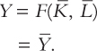
To this analysis, let’s add what we learned about the supply of goods and services in Section 3-1. There we saw that the factors of production and the production function determine the quantity of output supplied to the economy:
Now let’s combine these equations describing the supply and demand for output. If we substitute the consumption function and the investment function into the national accounts identity, we obtain
Y = C(Y – T) + I(r) + G.
Because the variables G and T are fixed by policy, and the level of output Y is fixed by the factors of production and the production function, we can write
This equation states that the supply of output equals its demand, which is the sum of consumption, investment, and government purchases.
Notice that the interest rate r is the only variable not already determined in the last equation. This is because the interest rate still has a key role to play: it must adjust to ensure that the demand for goods equals the supply. The greater the interest rate, the lower the level of investment, and thus the lower the demand for goods and services, C + I + G. If the interest rate is too high, investment is too low, and the demand for output falls short of the supply. If the interest rate is too low, investment is too high, and the demand exceeds the supply. At the equilibrium interest rate, the demand for goods and services equals the supply.
This conclusion may seem somewhat mysterious: How does the interest rate gets to the level that balances the supply and demand for goods and services? The best way to answer this question is to consider how financial markets fit into the story.
Equilibrium in the Financial Markets: The Supply and Demand for Loanable Funds
71
Because the interest rate is the cost of borrowing and the return to lending in financial markets, we can better understand the role of the interest rate in the economy by thinking about the financial markets. To do this, rewrite the national accounts identity as
Y – C – G = I.
The term Y – C – G is the output that remains after the demands of consumers and the government have been satisfied; it is called national saving or simply saving (S). In this form, the national accounts identity shows that saving equals investment.
To understand this identity more fully, we can split national saving into two parts—one part representing the saving of the private sector and the other representing the saving of the government:
(Y – T – C) + (T – G) = I.
The term (Y – T – C) is disposable income minus consumption, which is private saving. The term (T – G) is government revenue minus government spending, which is public saving. (If government spending exceeds government revenue, the government runs a budget deficit, and public saving is negative.) National saving is the sum of private and public saving. The circular flow diagram in Figure 3-1 reveals an interpretation of this equation: this equation states that the flows into the financial markets (private and public saving) must balance the flows out of the financial markets (investment).
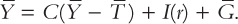
To see how the interest rate brings financial markets into equilibrium, substitute the consumption function and the investment function into the national accounts identity:
Y – C(Y – T) – G = I(r).
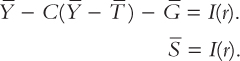
Next, note that G and T are fixed by policy and Y is fixed by the factors of production and the production function:
72
The left-hand side of this equation shows that national saving depends on income Y and the fiscal policy variables G and T. For fixed values of Y, G, and T, national saving S is also fixed. The right-hand side of the equation shows that investment depends on the interest rate.
Figure 3-8 graphs saving and investment as a function of the interest rate. The saving function is a vertical line because in this model saving does not depend on the interest rate (we relax this assumption later). The investment function slopes downward: the higher the interest rate, the fewer investment projects are profitable.
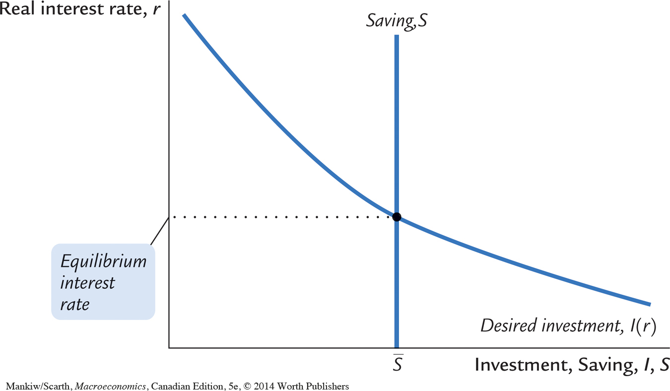
From a quick glance at Figure 3-8, one might think it was a supply and demand diagram for a particular good. In fact, saving and investment can be interpreted in terms of supply and demand. In this case, the “good” is loanable funds, and its “price” is the interest rate. Saving is the supply of loanable funds—households lend their saving to investors or deposit their saving in a bank that then loans the funds out. Investment is the demand for loanable funds—investors borrow from the public directly by selling bonds or indirectly by borrowing from banks. Because investment depends on the interest rate, the quantity of loanable funds demanded also depends on the interest rate.
The interest rate adjusts until the amount that firms want to invest equals the amount that households want to save. If the interest rate is too low, investors want more of the economy’s output than households want to save. Equivalently, the quantity of loans demanded exceeds the quantity supplied. When this happens, the interest rate rises. Conversely, if the interest rate is too high, households want to save more than firms want to invest; because the quantity of loans supplied is greater than the quantity demanded, the interest rate falls. The equilibrium interest rate is found where the two curves cross. At the equilibrium interest rate, households’ desire to save balances firms’ desire to invest, and the quantity of loans supplied equals the quantity demanded.
73
FYI
The Growing Gap Between Rich and Poor
The approximate constancy of the labour and capital shares of national income, which we observed in the Canadian data earlier in this chapter, has a straightforward implication: the distribution of income between workers and owners of capital has not radically changed over the course of history. There is, however, another way to look at the data on income distribution that shows more substantial changes. If we look within labour income, we find that the gap between the earnings of high-wage workers and the earnings of low-wage workers has grown substantially since the 1970s. As a result, income inequality is greater today than it was four decades ago; the same pattern is found in many western countries.
What has caused this growing income disparity between rich and poor? Economists do not have a definitive answer, but one diagnosis comes from economists Claudia Goldin and Lawrence Katz in their book The Race Between Education and Technology (Cambridge, Mass.: Belknap Press, 2011). Their bottom line is that ‘‘the sharp rise in inequality was largely due to an educational slowdown.’’
According to Goldin and Katz, for the past century technological progress has been a steady force that has not only increased average living standards, but has also increased the demand for skilled workers relative to unskilled workers. Skilled workers are needed to apply and manage new technologies, while less skilled workers are more likely to become obsolete.
For much of the 20th century, however, skill-biased technological change was outpaced by advances in educational attainment. In other words, while technological progress increased the demand for skilled workers, our educational system increased the supply of them even faster. As a result, skilled workers did not benefit disproportionately from economic growth.
But recently things have changed. Over the last several decades, technological advance has kept up its pace, while educational advancement has slowed down. Because growth in the supply of skilled workers has slowed, their wages have grown relative to those of the unskilled. This is evident in Goldin and Katz’s estimates of the financial return to education. In 1980, each year of college raised a person’s wage by 7.6 percent. In 2005, each year of college yielded an additional 12.9 percent. Over this time period, the rate of return from each year of graduate school has risen even more—from 7.3 to 14.2 percent.
The implication of this analysis for public policy is that reversing the rise in income inequality will likely require putting more of society’s resources into education (which economists call human capital). The implication for personal decision making is that college and graduate school are investments well worth making.
Changes in Saving: The Effects of Fiscal Policy
We can use our model to show how fiscal policy affects the economy. When the government changes its spending or the level of taxes, it affects the demand for the economy’s output of goods and services and alters national saving, investment, and the equilibrium interest rate.
An Increase in Government Purchases Consider first the effects of an increase in government purchases by an amount ΔG. The immediate impact is to increase the demand for goods and services by ΔG. But since total output is fixed by the factors of production, the increase in government purchases must be met by a decrease in some other category of demand. Since disposable income Y – T is unchanged, consumption C is unchanged as well. The increase in government purchases must be met by an equal decrease in investment.
74
To induce investment to fall, the interest rate must rise. Hence, the increase in government purchases causes the interest rate to increase and investment to decrease. Government purchases are said to crowd out investment.
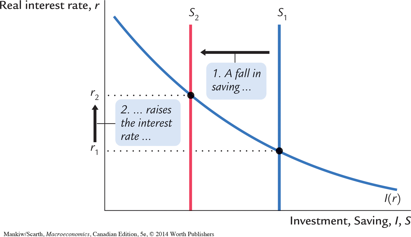
To grasp the effects of an increase in government purchases, consider the impact on the market for loanable funds. Since the increase in government purchases is not accompanied by an increase in taxes, the government finances the additional spending by borrowing—that is, by reducing public saving. Since private saving is unchanged, this government borrowing reduces national saving. As Figure 3-9 shows, a reduction in national saving is represented by a leftward shift in the supply of loanable funds available for investment. At the initial interest rate, the demand for loans exceeds the supply. The equilibrium interest rate rises to the point where the investment schedule crosses the new saving schedule. Thus, an increase in government purchases causes the interest rate to rise from r1 to r2.
CASE STUDY
Wars and Interest Rates in the United Kingdom, 1730–1920
Wars are traumatic—both for those who fight them and for a nation’s economy. Because the economic changes accompanying them are often large, wars provide a natural experiment with which economists can test their theories. We can learn about the economy by seeing how in wartime the endogenous variables respond to the major changes in the exogenous variables.
75
One exogenous variable that changes substantially in wartime is the level of government purchases. Figure 3-10 shows military spending as a percentage of GDP for the United Kingdom from 1730 to 1919. This graph shows, as one would expect, that government purchases rose suddenly and dramatically during the eight wars of this period.
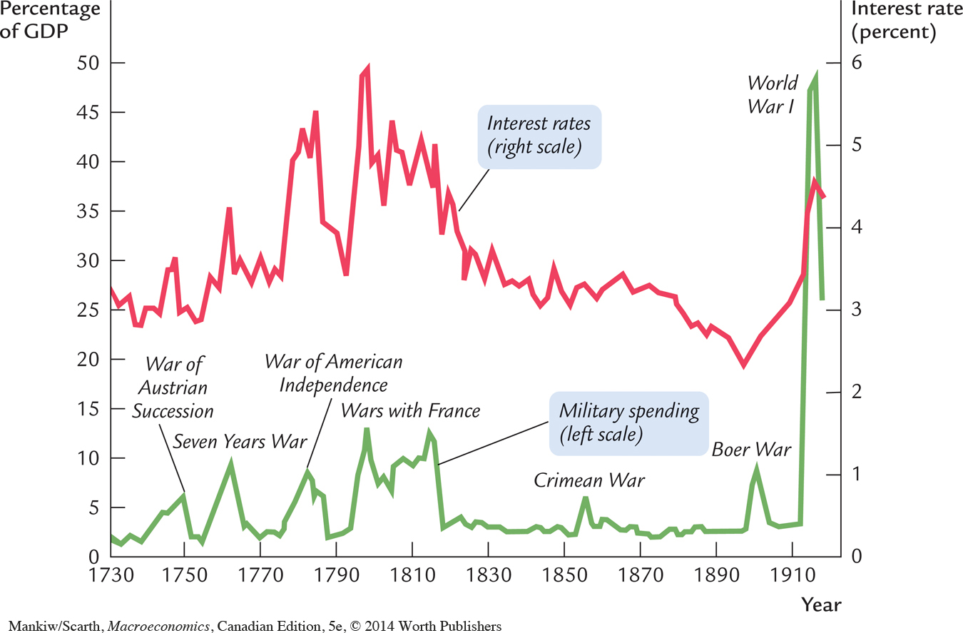
Our model predicts that this wartime increase in government purchases—and the increase in government borrowing to finance the wars—should have raised the demand for goods and services, reduced the supply of loanable funds, and raised the interest rate. To test this prediction, Figure 3-10 also shows the interest rate on long-term government bonds, called consols in the United Kingdom. A positive association between military purchases and interest rates is apparent in this figure. These data support the model’s prediction: interest rates do tend to rise when government purchases increase.7
76
One problem with using wars to test theories is that many economic changes may be occurring at the same time. For example, in World War II, while government purchases increased dramatically, rationing also restricted consumption of many goods. In addition, the risk of defeat in the war and default by the government on its debt presumably increases the interest rate the government must pay. Economic models predict what happens when one exogenous variable changes and all the other exogenous variables remain constant. In the real world, however, many exogenous variables may change at once. Unlike controlled laboratory experiments, the natural experiments on which economists must rely are not always easy to interpret. 
A Decrease in Taxes Now consider a reduction in taxes of ΔT. The immediate impact of the tax cut is to raise disposable income and thus to raise consumption. Disposable income rises by ΔT, and consumption rises by an amount equal to ΔT times the marginal propensity to consume MPC. The higher the MPC, the greater the impact of the tax cut on consumption.
Since the economy’s output is fixed by the factors of production and the level of government purchases is fixed by the government, the increase in consumption must be met by a decrease in investment. For investment to fall, the interest rate must rise. Hence, a reduction in taxes, like an increase in government purchases, crowds out investment and raises the interest rate.
We can also analyze the effect of a tax cut by looking at saving and investment. Since the tax cut raises disposable income by ΔT, consumption goes up by MPC × ΔT. National saving S, which equals Y – C – G, falls by the same amount as consumption rises. As in Figure 3-9, the reduction in saving shifts the supply of loanable funds to the left, which increases the equilibrium interest rate and crowds out investment.
CASE STUDY
Fiscal Policy in the 1980s and 1990s
One of the most dramatic economic events in recent history was the large change in fiscal policies of most Western countries in the latter three decades of the twentieth century. Before this period, all governments had run deficits during numerous short intervals of time. But governments had often run surpluses as well, so that, over the longer run, there was not a large increase in their national debts. Starting in the mid-1970s, however, the excess of government spending over tax revenues increased by a wide margin, and this gap became a permanent fixture of fiscal policy. It was not until the mid-1990s that deficits were worked down.
As our model predicts, this change in fiscal policy led to higher world interest rates and lower levels of saving. In Canada’s case, the real interest rate (the difference between the yield on government bonds and the inflation rate) rose from 0.8 percent in the 1960–1975 period to 3.9 percent in the 1976–1993 period. Total saving in Canada averaged 10 percent of national income in the 1960–1975 period, and only 2 percent in the early 1990s.8 The change in fiscal policy in the 1980s certainly had the effects that our simple model of the economy predicts.
Changes in Investment Demand
77
So far, we have discussed how fiscal policy can change national saving. We can also use our model to examine the other side of the market—the demand for investment. In this section we look at the causes and effects of changes in investment demand.
One reason investment demand might increase is technological innovation. Suppose, for example, that someone invents a new technology, such as the railroad or the computer. Before a firm or household can take advantage of the innovation, it must buy investment goods. The invention of the railroad had no value until railroad cars were produced and tracks were laid. The idea of the computer was not productive until computers were manufactured. Thus, technological innovation leads to an increase in investment demand.
Investment demand may also change because the government encourages or discourages investment through the tax laws. For example, suppose that the government increases personal income taxes and uses the extra revenue to provide tax cuts for those who invest in new capital. Such a change in the tax laws makes more investment projects profitable and, like a technological innovation, increases the demand for investment goods.
Figure 3-11 shows the effects of an increase in investment demand. At any given interest rate, the demand for investment goods (and also for loans) is higher. This increase in demand is represented by a shift in the investment schedule to the right. The economy moves from the old equilibrium, point A, to the new equilibrium, point B.
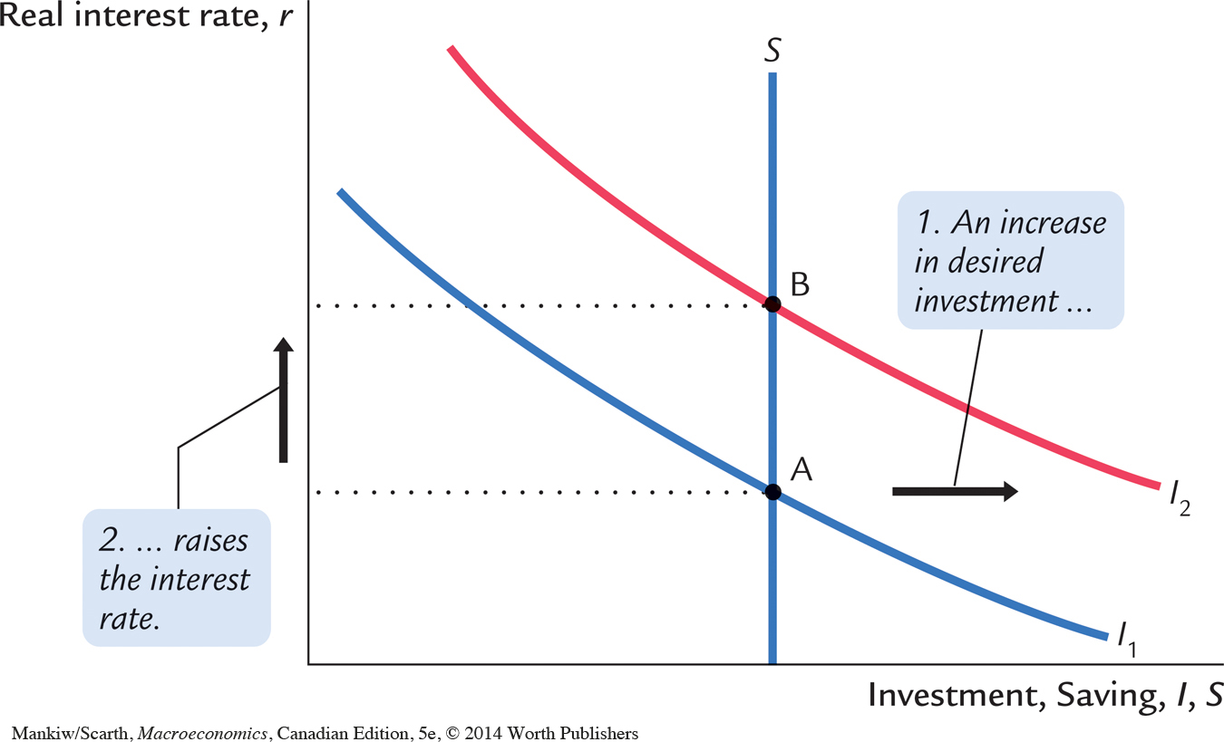
The surprising implication of Figure 3-11 is that the equilibrium amount of investment is unchanged. Under our assumptions, the fixed level of saving determines the amount of investment; in other words, there is a fixed supply of loans. An increase in investment demand merely raises the equilibrium interest rate.
78
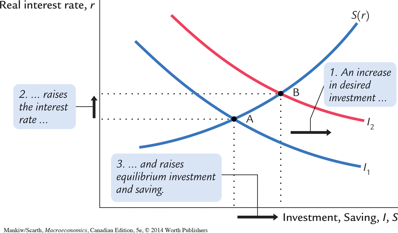
We would reach a different conclusion, however, if we modified our simple consumption function and allowed consumption (and its flip side, saving) to depend on the interest rate. Because the interest rate is the return to saving (as well as the cost of borrowing), a higher interest rate might reduce consumption and increase saving. If so, the saving schedule would be upward sloping, as it is in Figure 3-12, rather than vertical.
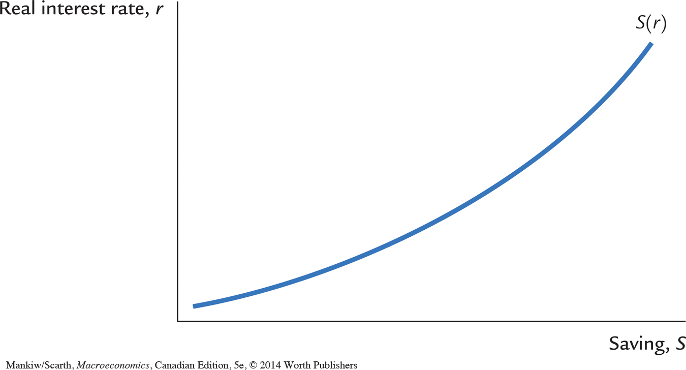
With an upward-sloping saving schedule, an increase in investment demand would raise both the equilibrium interest rate and the equilibrium quantity of investment. Figure 3-13 shows such a change. The increase in the interest rate causes households to consume less and save more. The decrease in consumption frees resources for investment.