mankiwscarth5e

3.5 Conclusion

In this chapter we have developed a model that explains the production, distribution, and allocation of the economy’s output of goods and services. Because the model incorporates all the interactions illustrated in the circular flow diagram in Figure 3-1, it is sometimes called a general equilibrium model. The model emphasizes how prices adjust to equilibrate supply and demand. Factor prices equilibrate factor markets. The interest rate equilibrates the supply and demand for goods and services (or, equivalently, the supply and demand for loanable funds).

Throughout the chapter, we have discussed various applications of the model. The model can explain how income is divided among the factors of production and how factor prices depend on factor supplies. We have also used the model to discuss how fiscal policy alters the allocation of output among its alternative uses—consumption, investment, and government purchases—and how it affects the equilibrium interest rate.

At this point it is useful to review some of the simplifying assumptions we have made in this chapter. In the following chapters we relax some of these assumptions to address a greater range of questions.

We have ignored the role of money, the asset with which goods and services are bought and sold. In Chapter 4 we discuss how money affects the economy and the influence of monetary policy.
We have assumed that there is no trade with other countries. In Chapter 5 we consider how international interactions affect our conclusions.
We have assumed that the labour force is fully employed. In Chapter 6 we examine the reasons for unemployment and see how public policy influences the level of unemployment.

80
We have assumed that the capital stock, the labour force, and the production technology (knowledge) are fixed. In Chapters 7 and 8 we see how changes over time in each of these lead to growth in the economy’s output of goods and services.
We have ignored the role of short-run sticky prices. In Chapters 9 through 14, we develop a model of short-run fluctuations that includes sticky prices. We then discuss how the model of short-run fluctuations relates to the model of national income developed in this chapter.

FYI

The Identification Problem

In our model, investment depends on the interest rate. The higher the interest rate, the fewer investment projects are profitable. The investment schedule therefore slopes downward.

Economists who look at macroeconomic data, however, usually fail to find an obvious association between investment and interest rates. In years when interest rates are high, investment is not always low. In years when interest rates are low, investment is not always high.

How do we interpret this finding? Does it mean that investment does not depend on the interest rate? Does it suggest that our model of saving, investment, and the interest rate is inconsistent with how the economy actually functions?

Luckily, we do not have to discard our model. The inability to find an empirical relationship between investment and interest rates is an example of the identification problem. The identification problem arises when variables are related in more than one way. When we look at data, we are observing a combination of these different relationships, and it is difficult to “identify” any one of them.

To understand this problem more concretely, consider the relationships among saving, investment, and the interest rate. Suppose, on the one hand, that all changes in the interest rate resulted from changes in saving—that is, from shifts in the saving schedule. Then, as shown in the left-hand side of panel (a) in Figure 3-14, all changes would represent movement along a fixed investment schedule. As the right-hand side of panel (a) shows, the data would trace out this investment schedule. Thus, we would observe a negative relationship between investment and interest rates.

Figure 3-14: FIGURE 3-14

Figure 3-14: Identifying the Investment Function When we look at data on interest rates r and investment l, what we find depends on which exogenous variables are changing. In panel (a), the saving schedule is shifting, perhaps because of changes in fiscal policy; we would observe a negative correlation between r and l. In panel (b), the investment schedule is shifting, perhaps because of technological innovations; we would observe a positive correlation between r and l. In the more realistic situation shown in panel (c), both schedules are shifting. In the data, we would observe no correlation between r and l, which is in fact what reseachers typically find.

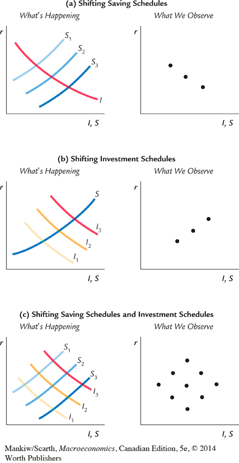
Suppose, on the other hand, that all changes in the interest rate resulted from technological innovations—that is, from shifts in the investment schedule. Then, as shown in panel (b), all changes would represent movements in the investment schedule along a fixed saving schedule. As the right-hand side of panel (b) shows, the data would reflect this saving schedule. Thus, we would observe a positive relationship between investment and interest rates.

In the real world, interest rates change sometimes because of shifts in the saving schedule and sometimes because of shifts in the investment schedule. In this mixed case, as shown in panel (c), a plot of the data would reveal no recognizable relation between interest rates and the quantity of investment, just as economists observe in actual data. The moral of the story is simple and is applicable to many other situations: the empirical relationship we expect to observe depends crucially on which exogenous variables we think are changing. Students who major in economics will learn how applied economists solve the identification problem in their statistics courses.

Before going on to these chapters, go back to the beginning of this one and make sure you can answer the four groups of questions about national income that begin the chapter.