5.2 Saving and Investment in a Small Open Economy
So far in our discussion of the international flows of goods and capital, we have rearranged accounting identities. That is, we have defined some of the variables that measure transactions in an open economy, and we have shown the links among these variables that follow from their definitions. Our next step is to develop a model that explains the behaviour of these variables. We can then use the model to answer questions such as how the trade balance responds to changes in policy.
Capital Mobility and the World Interest Rate
In a moment we present a model of the international flows of capital and goods. Because the trade balance equals the net capital outflow, which in turn equals saving minus investment, our model focuses on saving and investment. To develop this model, we use some elements that should be familiar from Chapter 3, but in contrast to the Chapter 3 model, we do not assume that the real interest rate equilibrates saving and investment. Instead, we allow the economy to run a trade deficit and borrow from other countries, or to run a trade surplus and lend to other countries.
136
If the real interest rate does not adjust to equilibrate saving and investment in this model, what does determine the real interest rate? We answer this question here by considering the simple case of a small open economy with perfect capital mobility. By “small’’ we mean that this economy is a small part of the world market and thus, by itself, can have only a negligible effect on the world interest rate. By “perfect capital mobility’’ we mean that residents of the country have full access to world financial markets. In particular, the government does not impede international borrowing or lending.
Because of this assumption of perfect capital mobility, the interest rate in our small open economy, r, must equal the world interest rate r*, the real interest rate prevailing in world financial markets, plus the risk premium θ associated with that particular economy. We write
r = r* + θ.
The small open economy takes the world real rate of interest as given, but its policies can have some effect on the risk premium.
Foreign lenders demand a risk premium when lending funds to Canadian firms and governments if they anticipate that the Canadian dollar may fall in value while the loan is outstanding. If that happens, foreign lenders will suffer a capital loss when they turn their earnings back into their own currency after the loan is repaid. To be compensated for that expected capital loss, lenders demand a yield that exceeds the world interest rate.
Figure 5-2 shows data for Canadian and American interest rates since 1962. Because we can interpret the U.S. interest rate as the “world” interest rate in our theoretical analysis, we see that the Canadian risk premium was quite small (and sometimes even negative) before 1975. Then, the risk premium widened somewhat, and many analysts attribute this to the fact that foreign lenders had become uneasy about both the size of Canadian government budget deficits and the prospect of prolonged political uncertainty surrounding the question of Quebec separation. Both these problems were expected to decrease the government’s resolve in maintaining zero inflation. If Canada inflates at a more rapid rate than other countries, the Canadian dollar has to fall in value to keep Canada’s exports from being priced out of foreign markets. With the federal and most provincial budget deficits eliminated by the end of the 1990s, with the perception that Quebec separation had become less likely, and with increased certainty concerning the Bank of Canada’s commitment to low inflation, the risk premium has been virtually eliminated in recent years.
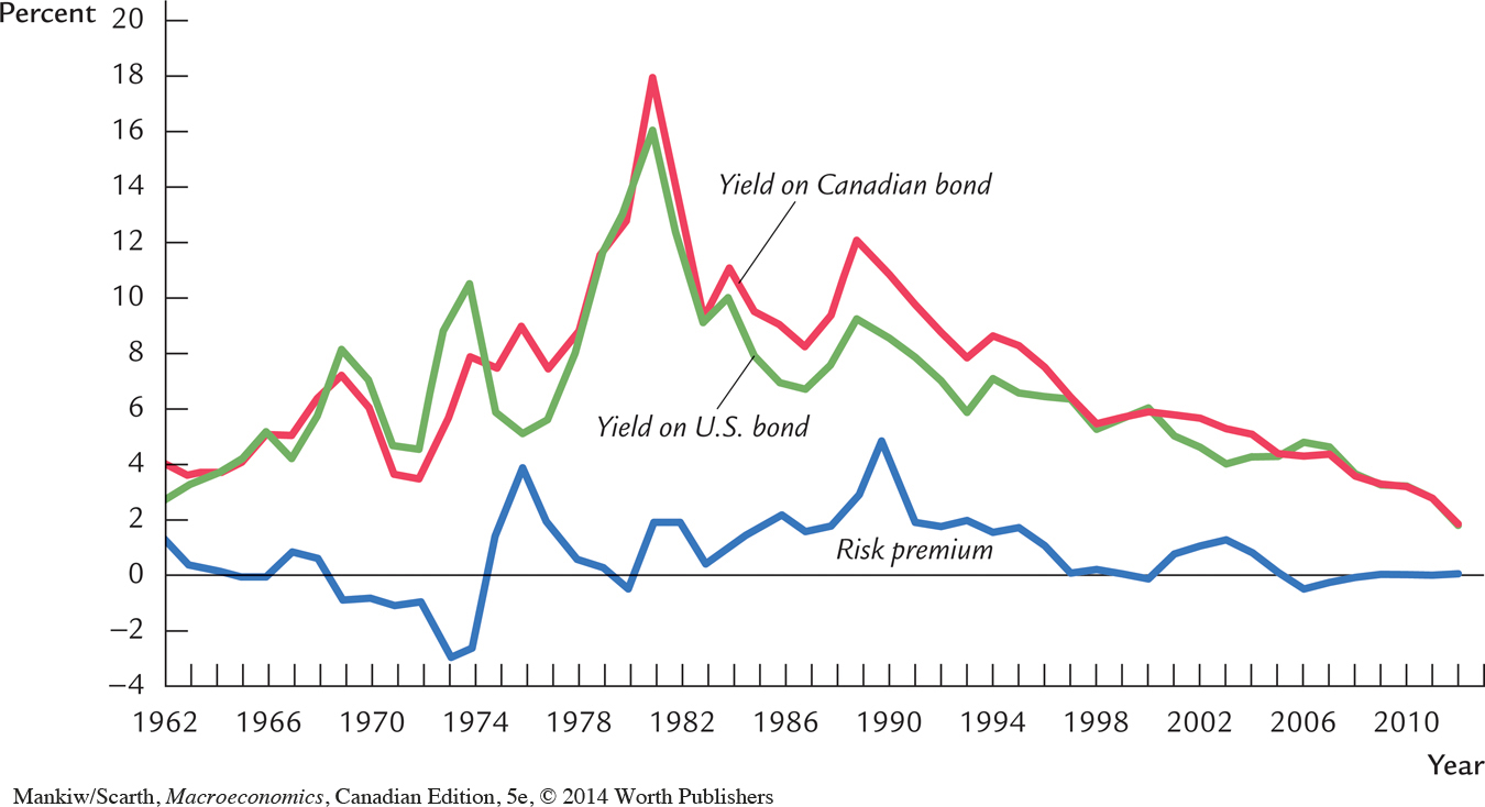
The interest rate differential shown in Figure 5-2 involves many short-run variations. These variations cannot be explained by longer-run issues, such as trends in political uncertainty. Instead, they are a result of the fact that it takes some time for international lenders to react to yield differentials. For example, if the Canadian interest rate rises above the American yield, it takes some time for lenders to notice that there is a substantial payoff to rearranging their bond holdings. Then, they must sell bonds in the rest of the world to obtain the funds necessary to buy Canadian bonds. Only after enough lenders have made this switch will the price paid for Canadian bonds be bid up sufficiently to force the effective yield earned by new buyers back down to equality with opportunities elsewhere. It is not surprising, therefore, that there are short-run departures from the equilibrium relationship.
137
For much of our discussion, we abstract from issues of longer term political uncertainty, and shorter term lags, and so we set the risk premium, θ, equal to 0. In other words, given the longer-run focus on economic issues in this chapter, we give little emphasis to the temporary departures from the equal yield relationship, and we assume
r = r*.
The small open economy takes its interest rate as given by the world real interest rate.
Let us discuss for a moment what determines the world real interest rate. In a closed economy, the equilibrium of domestic saving and domestic investment determines the interest rate. Barring interplanetary trade, the world economy is a closed economy. Therefore, the equilibrium of world saving and world investment determines the world interest rate. Our small open economy has a negligible effect on the world real interest rate because, being a small part of the world, it has a negligible effect on world saving and world investment. Hence, our small open economy takes the world interest rate as an exogenously given variable.
The Model
138
To build the model of the small open economy, we take three assumptions from Chapter 3:
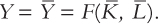
The economy’s output Y is fixed by the factors of production and the production function. We write this as
Consumption C is positively related to disposable income Y – T. We write the consumption function as
C = C(Y – T).
Investment I is negatively related to the real interest rate r. We write the investment function as
I = I(r).
These are the three key parts of our model. If you do not understand these relationships, review Chapter 3 before continuing.
We can now return to the accounting identity and write it as
NX = (Y – C – G) – I
= S – I.
Substituting the previous assumptions and the assumption that the interest rate equals the world interest rate, we obtain
This equation shows that the trade balance NX depends on variables that determine saving S and investment I. Because saving depends on fiscal policy (lower government purchases G or higher taxes T raise national saving) and investment depends on the world real interest rate r* (high interest rates make some investment projects unprofitable), the trade balance depends on these variables as well.
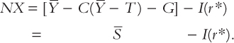
In Chapter 3 we graphed saving and investment as in Figure 5-3. In the closed economy studied in that chapter, the real interest rate adjusts to equilibrate saving and investment—that is, the real interest rate is found where the saving and investment curves cross. In the small open economy, however, the real interest rate equals the world real interest rate. The trade balance is determined by the difference between saving and investment at the world interest rate.
139
At this point, you might wonder about the mechanism that causes the trade balance to equal net foreign investment. The determinants of net foreign investment are easy to understand. When domestic saving falls short of domestic investment, domestic investors borrow from abroad; when saving exceeds investment, the excess is lent to other countries. But what causes those who import and export to behave in a way that ensures that the international flow of goods exactly balances this international flow of capital? For now we leave this question unanswered, but we return to it in Section 5-3 when we discuss the determination of exchange rates.
How Policies Influence the Trade Balance
Suppose that the economy begins in a position of balanced trade. That is, at the world interest rate, investment I equals saving S, and net exports NX equal zero. Let’s use our model to predict the effects of government policies at home and abroad.
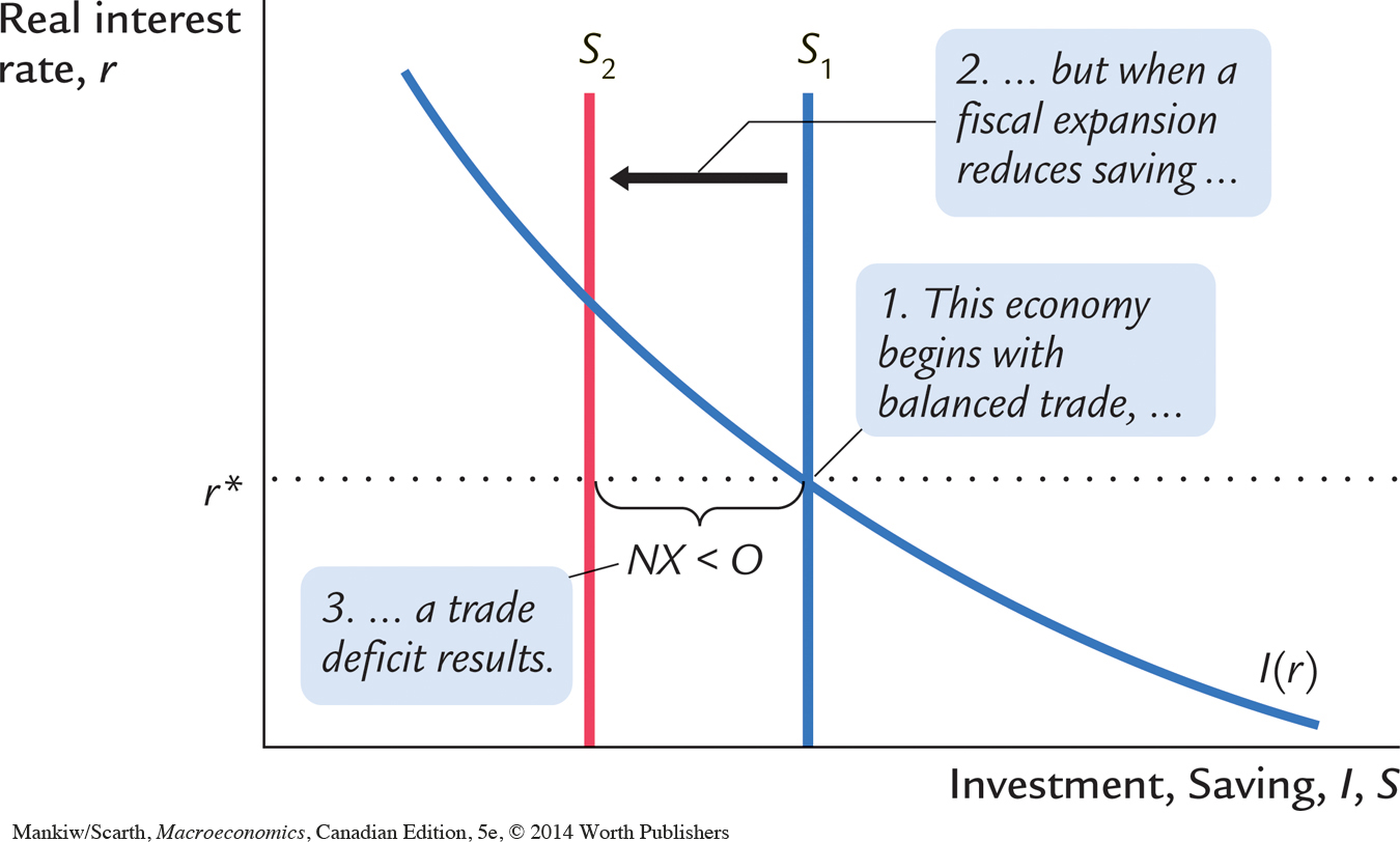
Fiscal Policy at Home Consider first what happens to the small open economy if the government expands domestic spending by increasing government purchases. The increase in G reduces national saving, because S = Y – C – G. With an unchanged world real interest rate, investment remains the same. Therefore, saving falls below investment, and some investment must now be financed by borrowing from abroad. Since NX = S – I, the fall in S implies a fall in NX. The economy now runs a trade deficit.
The same logic applies to a decrease in taxes. A tax cut lowers T, raises disposable income
Y – T, stimulates consumption, and reduces national saving. (Even though some of the tax cut finds its way into private saving, public saving falls by the full amount of the tax cut; in total, saving falls.) Since NX = S – I, the reduction in national saving in turn lowers NX.
140
Figure 5-4 illustrates these effects. A fiscal policy change that increases private consumption C or public consumption G reduces national saving (Y – C – G) and, therefore, shifts the vertical line that represents saving from S1 to S2. Because NX is the distance between the saving schedule and the investment schedule at the world interest rate, this shift reduces NX. Hence, starting from balanced trade, a change in fiscal policy that reduces national saving leads to a trade deficit. A change in fiscal policy that stimulates domestic investment spending has the same effect.
Fiscal Policy Abroad Consider now what happens to a small open economy when foreign governments increase their government purchases. If these foreign countries are a small part of the world economy, then their fiscal change has a negligible impact on other countries. But if these foreign countries are a large part of the world economy, their increase in government purchases reduces world saving and causes the world interest rate to rise, just as we saw in our closed economy model (remember, Earth is a closed economy).
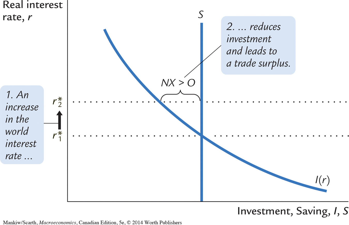
The increase in the world interest rate raises the cost of borrowing and, thus, reduces investment in our small open economy. Because there has been no change in domestic saving, saving S now exceeds investment I, and some of our saving begins to flow abroad. Since NX = S – I, the reduction in I must also increase NX. Hence, reduced saving abroad leads to a trade surplus at home.
Figure 5-5 illustrates how a small open economy starting from balanced trade responds to a foreign fiscal expansion. Because the policy change is occurring abroad, the domestic saving and investment schedules remain the same. The only change is an increase in the world interest rate from r1* to r2*. The trade balance is the difference between the saving and investment schedules; because saving exceeds investment at r2*, there is a trade surplus. Hence, starting from balanced trade, an increase in the world interest rate due to a fiscal expansion abroad leads to a trade surplus.
141
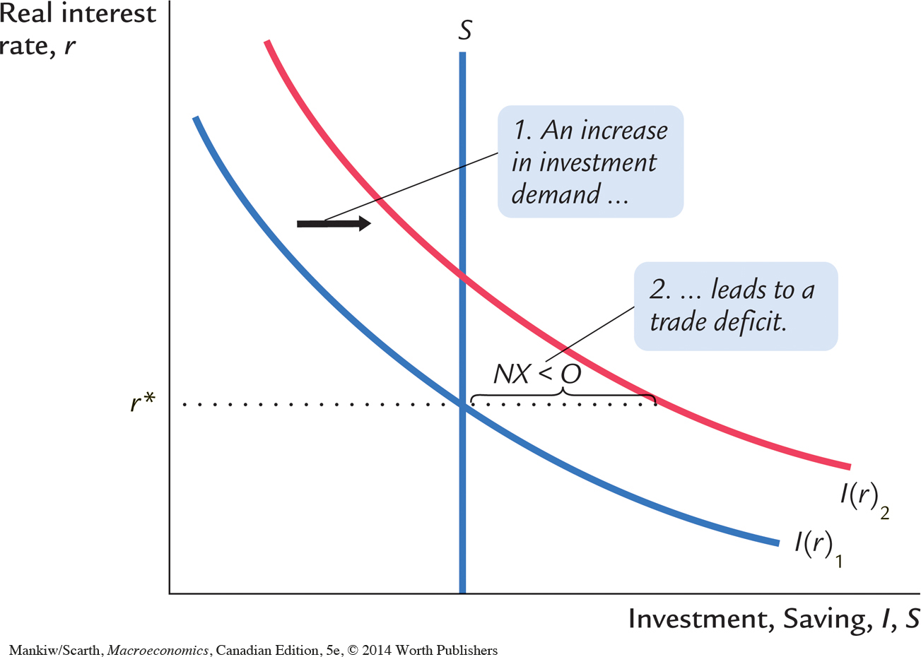
Shifts in Investment Demand Consider what happens to our small open economy if its investment schedule shifts outward—that is, if the demand for investment goods at every interest rate increases. This shift would occur if, for example, the government changed the tax laws to encourage investment by providing an investment tax credit. Figure 5-6 illustrates the impact of a shift in the investment schedule. At a given world interest rate, investment is now higher. Because saving is unchanged, some investment must now be financed by borrowing from abroad, which means net foreign investment is negative. Put differently, because NX = S – I, the increase in I implies a decrease in NX. Hence, an outward shift in the investment schedule causes a trade deficit.
Evaluating Economic Policy
142
Our model of the open economy shows that the flow of goods and services measured by the trade balance is inextricably connected to the flow of funds for capital accumulation. The net capital outflow is the difference between domestic saving and domestic investment. Thus, the impact of economic policies on the trade balance can always be found by examining their impact on domestic saving and domestic investment. Policies that increase investment or decrease saving tend to cause a trade deficit, and policies that decrease investment or increase saving tend to cause a trade surplus.
Our analysis of the open economy has been positive, not normative. That is, our analysis of how economic policies influence the international flows of capital and goods has not told us whether these policies are desirable. Evaluating economic policies and their impact on the open economy is a frequent topic of debate among economists and policymakers.
When a country runs a trade deficit, policymakers must confront the question of whether the trade deficit represents a national problem. Most economists view a trade deficit not as a problem in itself, but perhaps as a symptom of a problem. Trade deficits typically reflect a low saving rate. A low saving rate means that we are putting away less for the future. In a closed economy, low saving leads to low investment and a smaller future capital stock. In an open economy, low saving leads to a trade deficit and a growing foreign debt, which eventually must be repaid. In both cases, high current consumption leads to lower future consumption, implying that future generations bear the burden of low national saving.
Yet trade deficits are not always a reflection of economic malady. When poor rural economies develop into modern industrial economies, they sometimes finance their high levels of investment with foreign borrowing. In these cases, trade deficits are a sign of economic development. For example, South Korea ran large trade deficits throughout the 1970s, and it became one of the success stories of economic growth. The lesson is that one cannot judge economic performance from the trade balance alone. Instead, one must look at the underlying causes of the international flows.
CASE STUDY
The U.S. Trade Deficit
During the 1980s, 1990s, and early 2000s, the United States ran large trade deficits. Panel (a) of Figure 5-7 documents this experience by showing net exports as a percentage of GDP. The exact size of the trade deficit fluctuated over time, but it was large throughout these two and a half decades. In 2007, the trade deficit was $708 billion, or 5.1 percent of GDP. As accounting identities require, this trade deficit had to be financed by borrowing from abroad (or equivalently by selling U.S. assets abroad). During this period, the United States went from being the world’s largest creditor to the world’s largest debtor.
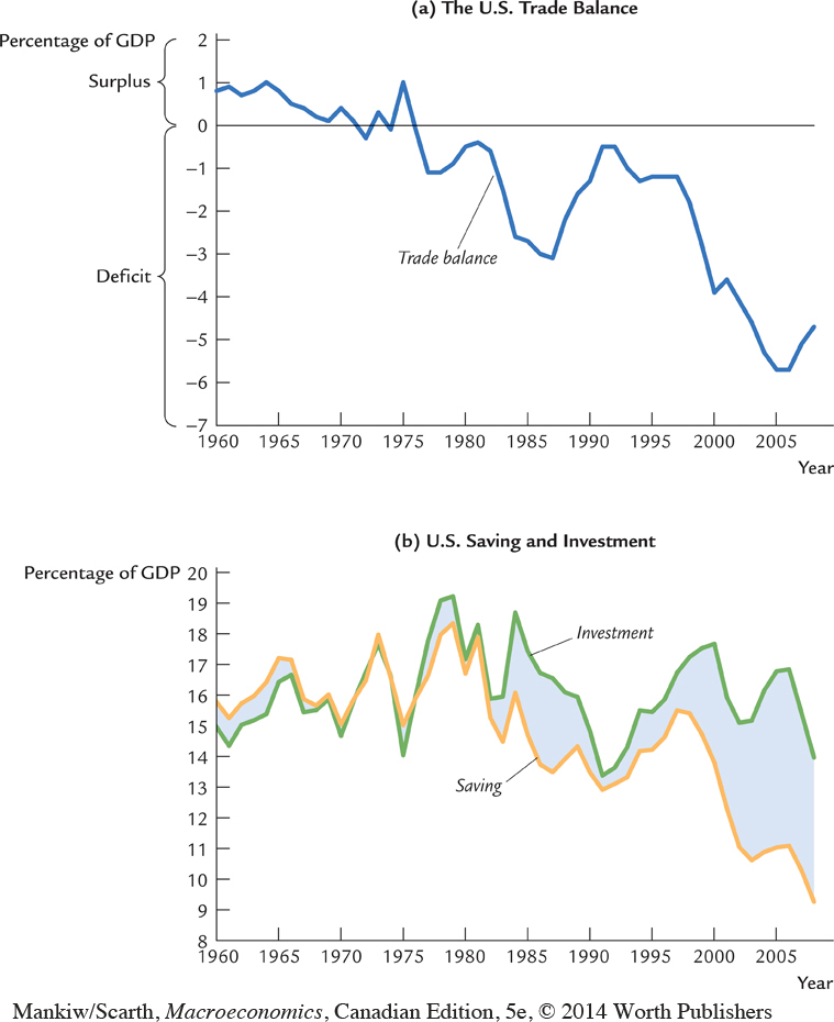
What caused the U.S. trade deficit? There is no single explanation. But to understand some of the forces at work, it helps to look at American national saving and domestic investment, as shown in panel (b) of the figure. Keep in mind that the trade deficit is the difference between saving and investment.
143
144
The start of the trade deficit coincided with a fall in national saving. This development can be explained by the expansionary fiscal policy in the 1980s. With the support of President Reagan, the U.S. Congress passed legislation in 1981 that substantially cut personal income taxes over the next three years. Because these tax cuts were not met with equal cuts in government spending, the federal budget went into deficit. These budget deficits were among the largest ever experienced in a period of peace and prosperity, and they continued long after Reagan left office. According to our model, such a policy should reduce national saving, thereby causing a U.S. trade deficit. In fact, that is exactly what happened. Because the government budget and trade balance went into deficit at roughly the same time, these shortfalls were called the twin deficits.
Things started to change in the 1990s, when the U.S. federal government got its fiscal house in order. The first President Bush and President Clinton both signed tax increases, while Congress kept a lid on spending. In addition to these policy changes, rapid productivity growth in the late 1990s raised incomes and thus further increased tax revenue. These developments moved the U.S. federal budget from deficit to surplus, which in turn caused national saving to rise.
Why didn’t the increase in national saving generate a shrinking trade deficit? The reason is that domestic investment spending rose at the same time. The likely explanation for this development is that the boom in information technology caused an expansionary shift in the U.S. investment function. Even though fiscal policy was pushing the trade deficit toward surplus, the investment boom was an even stronger force pushing the trade balance toward deficit.
In the early 2000s, fiscal policy once again put downward pressure on national saving. With the second President Bush in the White House, tax cuts were signed into law in 2001 and 2003, while the war on terror and in Iraq led to substantial increases in government spending. The federal government was again running budget deficits. National saving fell to historic lows, and the trade deficit reached historic highs.
A few years later, the trade deficit started to shrink somewhat as the economy experienced a substantial decline in housing prices (a phenomenon examined in case studies in Chapters 11 and 18). Lower housing prices reduced residential investment and made households poorer, inducing them to reduce consumption and increase saving. As a result, the trade deficit fell from 6.1 percent of GDP at its peak in the fourth quarter of 2005 to 4.9 percent in the third quarter of 2007.
The history of the U.S. trade deficit shows that this statistic, by itself, does not tell us much about what is happening in the economy. We have to look deeper at saving, investment, and the policies and events that cause them to change over time.1 No country can “solve” its trade deficit “problem” without achieving some combination of reducing its government budget deficit, increasing its rate of private saving, and decreasing its rate of investment spending.
145
It is interesting to interpret the rhetoric on both sides concerning the massive trade imbalance. One such imbalance that has been in the news recently concerns China and the United States. The United States is concerned about the large magnitude of the net surplus China has in the trade between the two nations. American politicians argue that the Chinese should raise the value of their currency to stimulate Chinese imports from the United States. This would help reduce the U.S. trade deficit, without the Americans’ having to make painful choices themselves. Like everyone else, the Americans find it difficult to make large cuts in their own government budget deficit or to make cuts in domestic investment (since these cuts lower capital accumulation and future living standards within the country). Knowledge of the twin deficits relationship allows us to understand the logic behind these trade disputes. 
CASE STUDY
Why Doesn’t Capital Flow to Poor Countries?
The U.S. trade deficit discussed in the previous case study represents a flow of capital into the United States from the rest of the world. What countries were the source of the capital flows? Because the world is a closed economy, the capital must be coming from countries that were running trade surpluses. In 2008, this group included many nations that were far poorer than the United States, such as Russia, Malaysia, Venezuela, and China. In these nations, saving exceeded investment in domestic capital. These countries were sending funds abroad to countries like the United States, where investment in domestic capital exceeded saving.
From one perspective, the direction of international capital flows is a paradox. Recall our discussion of production functions in Chapter 3. There, we established that an empirically realistic production function is the Cobb–Douglas form:
F(K,L) = A KαL1–α,
where K is capital, L is labour, A is a variable representing the state of technology, and α is a parameter that determines capital’s share of total income. For this production function, the marginal product of capital is
MPK = α A (K/L)α–1.
The marginal product of capital tells us how much more output an extra unit of capital would produce. Because α is capital’s share, it must be less than 1, so α –1 < 0. This means that an increase in K/L decreases MPK. In other words, holding other variables constant, the more capital a nation has, the less valuable an extra unit of capital is. This phenomenon of diminishing marginal product says that capital should be more valuable when capital is scarce.
This prediction, however, seems at odds with the international flow of capital represented by trade imbalances. Capital does not seem to flow to nations where it should be most valuable. Instead of capital-rich countries like the United States lending to capital-poor countries, we often observe the opposite. Why is that?
146
One reason is that there are important differences among nations other than their accumulation of capital. Poor nations have not only lower levels of capital accumulation (represented by K/L) but also inferior production capabilities (represented by the variable A). For example, compared to rich nations, poor nations may have less access to advanced technologies, lower levels of education (or human capital), or less efficient economic policies. Such differences could mean less output for given inputs of capital and labour; in the Cobb–Douglas production function, this is translated into a lower value of the parameter A. If so, then capital need not be more valuable in poor nations, even though capital is scarce.
A second reason why capital might not flow to poor nations is that property rights are often not enforced. Corruption is typically extensive; revolutions, coups, and expropriation of wealth are common; and governments often default on their debts. So, even if capital is more valuable in poor nations, foreigners may avoid investing their wealth there simply because they are afraid of losing it. Moreover, local investors face similar incentives. Imagine that you lived in a poor nation and you happened to be lucky enough to have wealth to invest; you might well decide that putting it in a safe country like the United States is your best option, even if the marginal product of capital is less there than in your home country.
Whichever of the two reasons is correct, the challenge for poor nations is to find ways to reverse the situation. If these nations offered the same production efficiency and legal protections as the U.S. economy, the direction of international capital flows would likely reverse. The U.S. trade deficit would become a trade surplus, and capital would flow to these emerging nations. Such a change would help the poor of the world escape poverty.2