5.3 Exchange Rates
Having examined the international flows of capital and of goods and services, we now extend the analysis by considering the prices that apply to these transactions. The exchange rate between two countries is the price at which residents of those countries trade with each other. In this section we first examine precisely what the exchange rate measures, and we then discuss how exchange rates are determined.
Nominal and Real Exchange Rates
Economists distinguish between two exchange rates: the nominal exchange rate and the real exchange rate. Let’s discuss each in turn and see how they are related.
The Nominal Exchange Rate The nominal exchange rate is the relative price of the currency of two countries. For example, if the exchange rate between the Canadian dollar and the Japanese yen is 100 yen per dollar, then you can exchange 1 dollar for 100 yen in world markets for foreign currency. A Japanese who wants to obtain dollars would pay 100 yen for each dollar she bought. A Canadian who wants to obtain yen would get 100 yen for each dollar he paid. When people refer to “the exchange rate’’ between two countries, they usually mean the nominal exchange rate.
147
FYI
How Newspapers Report the Exchange Rate
You can find exchange rates reported daily in many newspapers, although, increasingly, newspapers expect readers to look up exchange rates on the Internet. Alternatively, newspapers transfer users of their own web-based editions to the Bank of Canada exchange-rate website. To view that website, visit http://www.bank-banque-canada.ca/, then click on “English,” then “Rates and Statistics,” and then “Exchange Rates.” You then have many options, such as a currency converter for 56 currencies. The material reproduced in this box represents what was available on May 21, 2013, when the “US$/CAN$ closing rate summary” was chosen.
Notice that on that date, one U.S. dollar bought 1.0291 Canadian dollars. Often you will read or hear the exchange rate reported as the value of the Canadian dollar, not the value of the U.S. dollar—as it is here. This alternative measure is simply the inverse. On May 21, 2013, the value of the Canadian dollar in terms of U.S. dollars was (1/1.0291) = 0.9717, so the news media reported that the Canadian dollar was worth about 97 U.S. cents. As you can see, these two ways of reporting the exchange rate are equivalent ways of expressing the relative price of the two currencies. This book always expresses the exchange rate in units of foreign currency per Canadian dollar—the inverse of the basic practice followed on the Bank of Canada exchange-rate website. But the Bank does report our preferred definition in the column on the right.
You can see that the value of the Canadian dollar varies quite a lot. For example, in mid-2012, the U.S. dollar was higher (at $1.0397 Canadian), while three months later, the U.S. dollar was lower (at $0.968 Canadian). Since we are defining the value of the Canadian dollar as our exchange rate, we say that there was an appreciation in the value of our currency and exchange rate between June and September 2012.
| US$ to CAN$ | CAN$ to US$ | |
| Latest closing | (2013-05-17) – $1.0291 | 0.9717 |
| Past 12 months: | ||
| High | (2012-06-04) – $1.0397 | 0.9618 |
| Low | (2012-09-13) – $0.9683 | 1.0327 |
| From 1950 to present: | ||
| High | (2002-01-18) – $1.6125 | 0.6202 |
| Low | (2007-11-06) – $0.9215 | 1.0852 |
| Month | US$ to CAN$ | CAN$ to US$ |
| 2013-04 | 1.0075 | 0.9926 |
| 2013-03 | 1.0160 | 0.9843 |
| 2013-02 | 1.0314 | 0.9696 |
| 2013-01 | 0.9973 | 1.0027 |
| 2012-12 | 0.9949 | 1.0051 |
| 2012-11 | 0.9936 | 1.0064 |
| 2012-10 | 0.9990 | 1.0010 |
| 2012-09 | 0.9832 | 1.0171 |
| 2012-08 | 0.9857 | 1.0145 |
| 2012-07 | 1.0029 | 0.9971 |
| 2012-06 | 1.0181 | 0.9822 |
| 2012-05 | 1.0329 | 0.9681 |
Latest closing rate is updated at about 16:30 ET the same business day.
Source: Copyright © Bank of Canada.
148
The Real Exchange Rate The real exchange rate is the relative price of the goods of two countries. That is, the real exchange rate tells us the rate at which we can trade the goods of one country for the goods of another. The real exchange rate is sometimes called the terms of trade.
To see the relation between the real and nominal exchange rates, consider a single good produced in many countries: cars. Suppose a Canadian car costs $20,000 and a similar Japanese car costs 2,400,000 yen. To compare the prices of the two cars, we must convert them into a common currency. If a dollar is worth 100 yen, then the Canadian car costs 2,000,000 yen. Comparing the price of the Canadian car (2,000,000 yen) and the price of the Japanese car (2,400,000 yen), we conclude that the Canadian car costs five-sixths of what the Japanese car costs. In other words, at current prices, we can exchange 6 Canadian cars for 5 Japanese cars.
We can summarize our calculation above as follows:
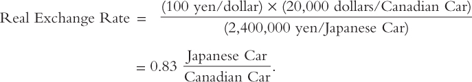
At these prices and this exchange rate, we obtain five-sixths of a Japanese car per Canadian car. More generally, we can write this calculation as

The rate at which we exchange foreign and domestic goods depends on the prices of the goods in the local currencies and on the rate at which the currencies are exchanged.
This calculation of the real exchange rate for a single good suggests how we should define the real exchange rate for a broader basket of goods. Let e be the nominal exchange rate (the number of yen per dollar), P be the price level in Canada (measured in dollars), and P* be the price level in Japan (measured in yen). Then the real exchange rate ϵ is
Real Exchange Rate = Nominal Exchange Rate × Ratio of Price Levels
ϵ = e x (P/P*).
The real exchange rate between two countries is computed from the nominal exchange rate and the price levels in the two countries. If the real exchange rate is high, foreign goods are relatively cheap, and domestic goods are relatively expensive. If the real exchange rate is low, foreign goods are relatively expensive, and domestic goods are relatively cheap.
The Real Exchange Rate and the Trade Balance
149
What macroeconomic influence does the real exchange rate exert? To answer this question, remember that the real exchange rate is nothing more than a relative price. Just as the relative price of hamburgers and pizza determines which you choose for lunch, the relative price of domestic and foreign goods affects the demand for these goods.
Suppose first that the real exchange rate is low. In this case, because domestic goods are relatively cheap, domestic residents will want to purchase fewer imported goods: they will buy Fords rather than Volkswagens, drink Coors rather than Heineken, and vacation in the Rockies rather than Europe. For the same reason, foreigners will want to buy many of our goods. As a result of both of these actions, the quantity of our net exports demanded will be high.
The opposite occurs if the real exchange rate is high. Because domestic goods are expensive relative to foreign goods, domestic residents will want to buy many imported goods, and foreigners will want to buy few of our goods. Therefore, the quantity of our net exports demanded will be low.
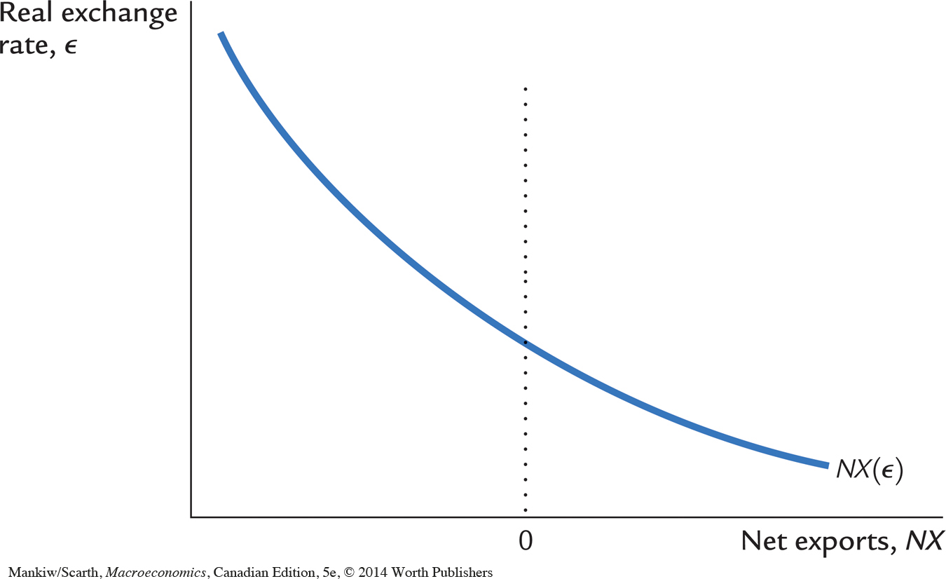
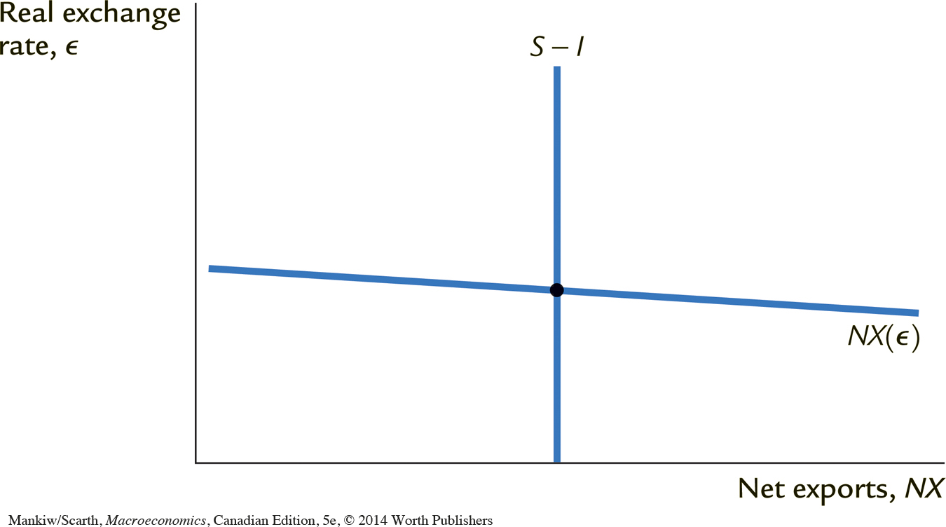
We write this relationship between the real exchange rate and net exports as
NX = NX(ϵ).
This equation states that net exports are a function of the real exchange rate. Figure 5-8 illustrates this negative relationship between the trade balance and the real exchange rate.
150
CASE STUDY
Traders Respond to the Exchange Rate
The value of the Canadian dollar has fluctuated rather dramatically over the years. Back in 1986, the Canadian dollar bought only $0.72 U.S. By 1991, Canadian currency had so increased in value that it bought $0.87 U.S. Then, by the end of the century, the Canadian dollar had dropped again, and it could only bring $0.69 U.S. in trades on the foreign exchange market. In 2006, the value of the Canadian dollar was back up to $0.90 U.S., and it peaked at $1.09 U.S. in November 2007. As this book was going to press, the Canadian dollar was back at $0.87 U.S. Given this pattern, it is not surprising that trade across the Canada–United States border has been affected.
The phenomenon of “cross-border shopping” has been widely discussed in the media. While the Canadian dollar was high in value, many Canadians made one-day trips to border towns in the United States to capitalize on the bargains that could be had in the “warehouse malls” there. On weekend days, there were tremendous traffic jams at the border, as cross-border shoppers swamped the facilities at the customs points. Canadian retailers pleaded with governments to “do something” to help keep their businesses from failing (and many did fail). By the mid-1990s, the cross-border shopping “problem” had all but disappeared. Indeed, the media carried stories about how the traffic had started to go the other way. Americans had started to realize how much their currency then could buy in Canada. These developments are perfectly predictable, given the large changes in the exchange rate. Cross-border shopping is just one more instance of households and firms choosing to consume more of the items that are available at lower relative prices.
The variation in the Canada–United States exchange rate during this period also caused controversy regarding the Canada–U.S. Free Trade Agreement, which came into effect in January 1989. From Canada’s point of view, one of the purposes of the deal was to allow Canadian firms to gain better access to the large U.S. market (for selling Canadian goods). But there were competing effects on the competitiveness of Canadian firms. The removal of U.S. tariffs that formed part of the Free Trade Agreement made Canadian firms more competitive, but the fact that the Canadian dollar was so much more expensive to buy in 1989 (than it was in 1986) made Canadian firms less competitive. Many analysts argue that the high value of the Canadian exchange rate at that time delayed the benefits that Canada should have obtained from signing the trade deal.
It is not just trade with the United States that is affected by exchange-rate changes. In 1990, 1 Canadian dollar bought 123 Japanese yen. By 1994, the Canadian dollar had fallen to the point where it could only buy 75 yen. Consumers responded in the obvious way. Back in 1990, North American car manufacturers were suffering losses in sales and were offering large “cashbacks” to attract customers. North American sales of Japanese cars, on the other hand, were booming. Then, by 1994, the Japanese manufacturers were suffering large drops in car sales, and the North American car sales had recovered. The fortunes of these domestic car manufacturers subsequently reversed again, as the Canadian dollar rose in the early years of the present century.
The point of these stories is that the negative slope we have shown for the net export schedule in Figure 5-8 should not be controversial. 
The Determinants of the Real Exchange Rate
151
We now have all the pieces needed to construct a model that explains what factors determine the real exchange rate. In particular, we combine the relationship between net exports and the real exchange rate we just discussed with the model of the trade balance we developed earlier in the chapter. We can summarize the analysis as follows:
The real exchange rate is related to net exports. When the real exchange rate is lower, domestic goods are less expensive relative to foreign goods, and net exports are greater.
The trade balance (net exports) must equal net foreign investment, which in turn equals saving minus investment. Saving is fixed by the consumption function and fiscal policy; investment is fixed by the investment function and the world interest rate.
Figure 5-9 illustrates these two conditions. The line showing the relationship between net exports and the real exchange rate slopes downward because a low real exchange rate—a “competitive” domestic economy—makes domestic goods relatively inexpensive. The line representing the excess of saving over investment, S – I, is vertical because neither saving nor investment depends on the real exchange rate. The crossing of these two lines determines the equilibrium exchange rate.
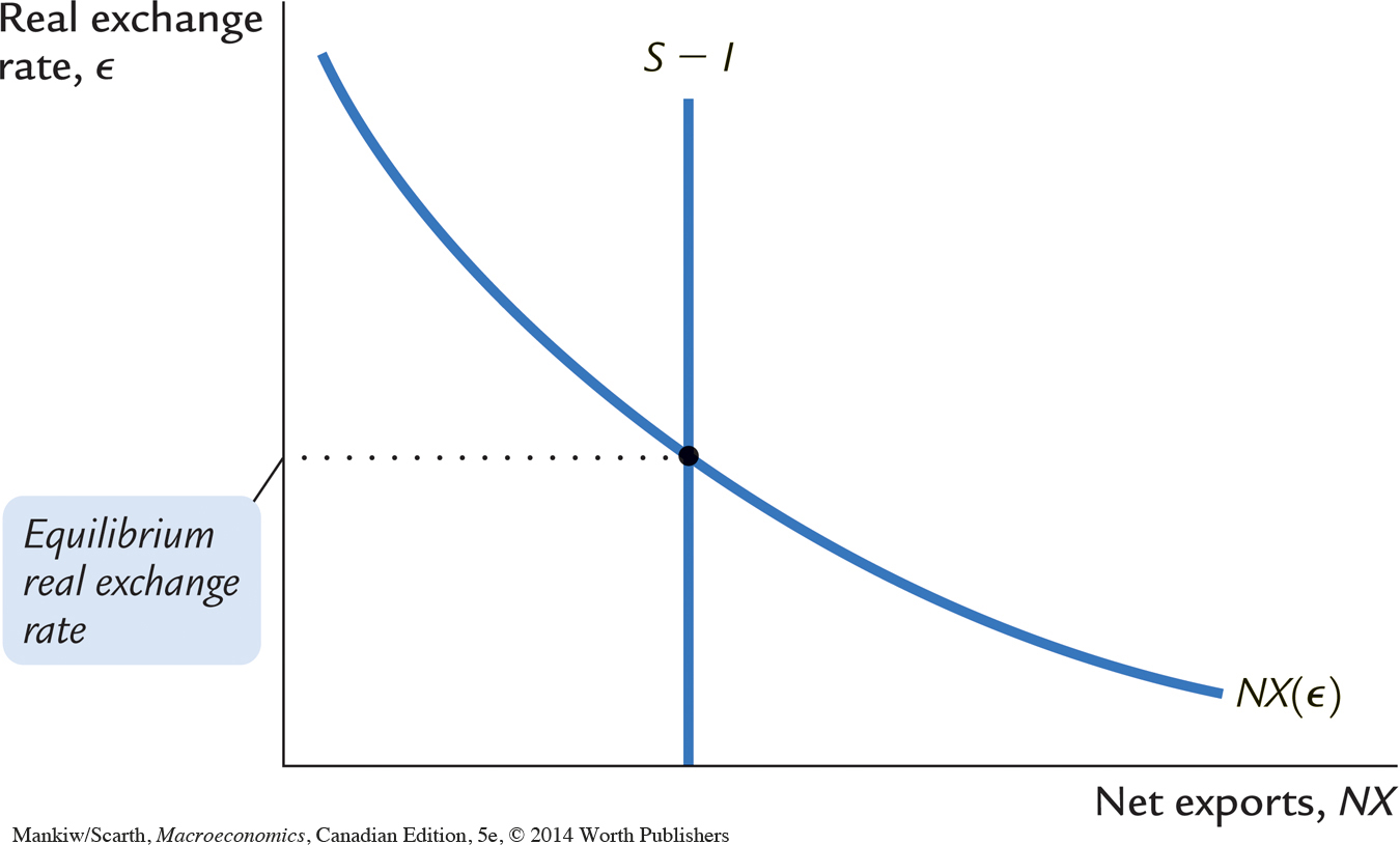
Figure 5-9 looks like an ordinary supply-and-demand diagram. In fact, you can think of this diagram as representing the supply and demand for foreign-currency exchange. The vertical line, S – I, represents the excess of domestic saving over domestic investment, and thus the supply of Canadian dollars to be exchanged into foreign currency and invested abroad. The downward-sloping line, NX, represents the net demand for Canadian dollars coming from foreigners who want Canadian dollars to buy our goods. At the equilibrium real exchange rate, the supply of Canadian dollars available for net foreign investment balances the demand for dollars by foreigners buying our net exports
How Policies Influence the Real Exchange Rate
152
We can use this model to show how the changes in economic policy we discussed earlier affect the real exchange rate.
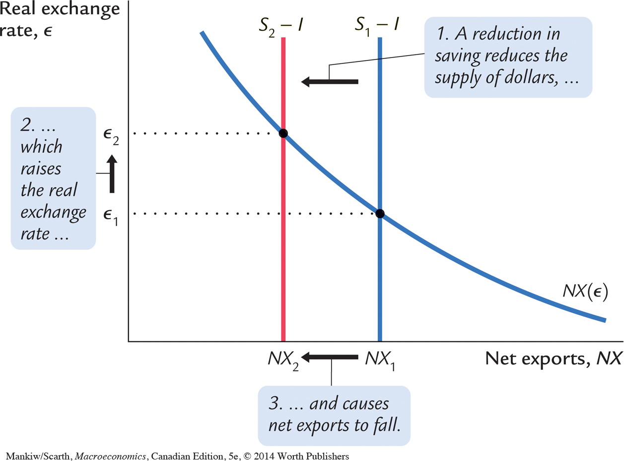
Fiscal Policy at Home What happens to the real exchange rate if the government reduces national saving by increasing government purchases or cutting taxes? As we discussed earlier, this reduction in saving lowers S – I and thus NX. That is, the reduction in saving causes a trade deficit.
Figure 5-10 shows how the equilibrium real exchange rate adjusts to ensure that NX falls. The change in policy shifts the vertical S – I line to the left, lowering the supply of Canadian dollars to be invested abroad. The lower supply causes the equilibrium real exchange rate to rise from ϵ1 to ϵ2—that is, the dollar becomes more valuable. Because of the rise in the value of the dollar, domestic goods become more expensive relative to foreign goods, which causes exports to fall and imports to rise. The change in exports and the change in imports both act to reduce net exports.
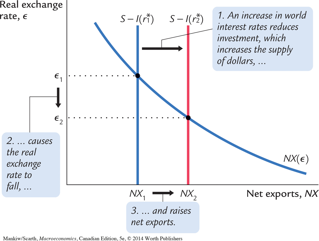
Fiscal Policy Abroad What happens to the real exchange rate if foreign governments increase government purchases or cut taxes? This change in fiscal policy reduces world saving and raises the world interest rate. The increase in the world interest rate reduces domestic investment I, which raises S – I and thus NX. That is, the increase in the world interest rate causes a trade surplus.
Figure 5-11 shows that this change in policy shifts the vertical S – I line to the right, raising the supply of Canadian dollars to be invested abroad. The equilibrium real exchange rate falls. That is, the dollar becomes less valuable, and domestic goods become less expensive relative to foreign goods.
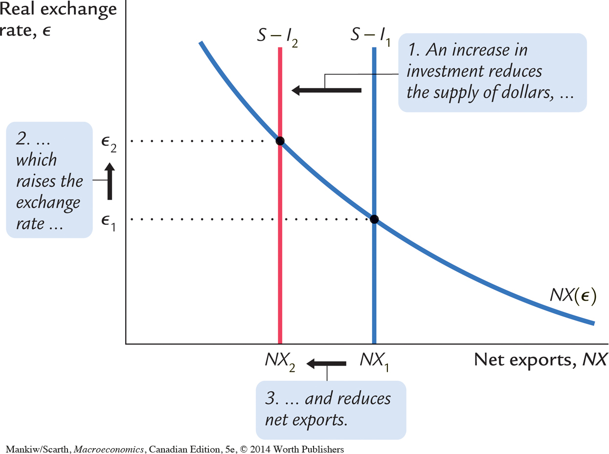
Shifts in Investment Demand What happens to the real exchange rate if investment demand at home increases, perhaps because the Canadian government introduces an investment tax credit? At the given world interest rate, the increase in investment demand leads to higher investment. A higher value of I means lower values of S – I and NX. That is, the increase in investment demand causes a trade deficit.
153
Figure 5-12 shows that the increase in investment demand shifts the vertical S − I line to the left, reducing the supply of Canadian dollars to be invested abroad. The equilibrium real exchange rate rises. Hence, when the investment tax credit makes investing in Canada more attractive, it also increases the value of the Canadian dollars necessary to make these investments. When the dollar appreciates, domestic goods become more expensive relative to foreign goods, and net exports fall.
The Effects of Trade Policies
154
Now that we have a model that explains the trade balance and the real exchange rate, we have the tools to examine the macroeconomic effects of trade policies. Trade policies, broadly defined, are policies designed to influence directly the amount of goods and services exported or imported. Most often, trade policies take the form of protecting domestic industries from foreign competition—either by placing a tax on foreign imports (a tariff) or restricting the amount of goods and services that can be imported (a quota).
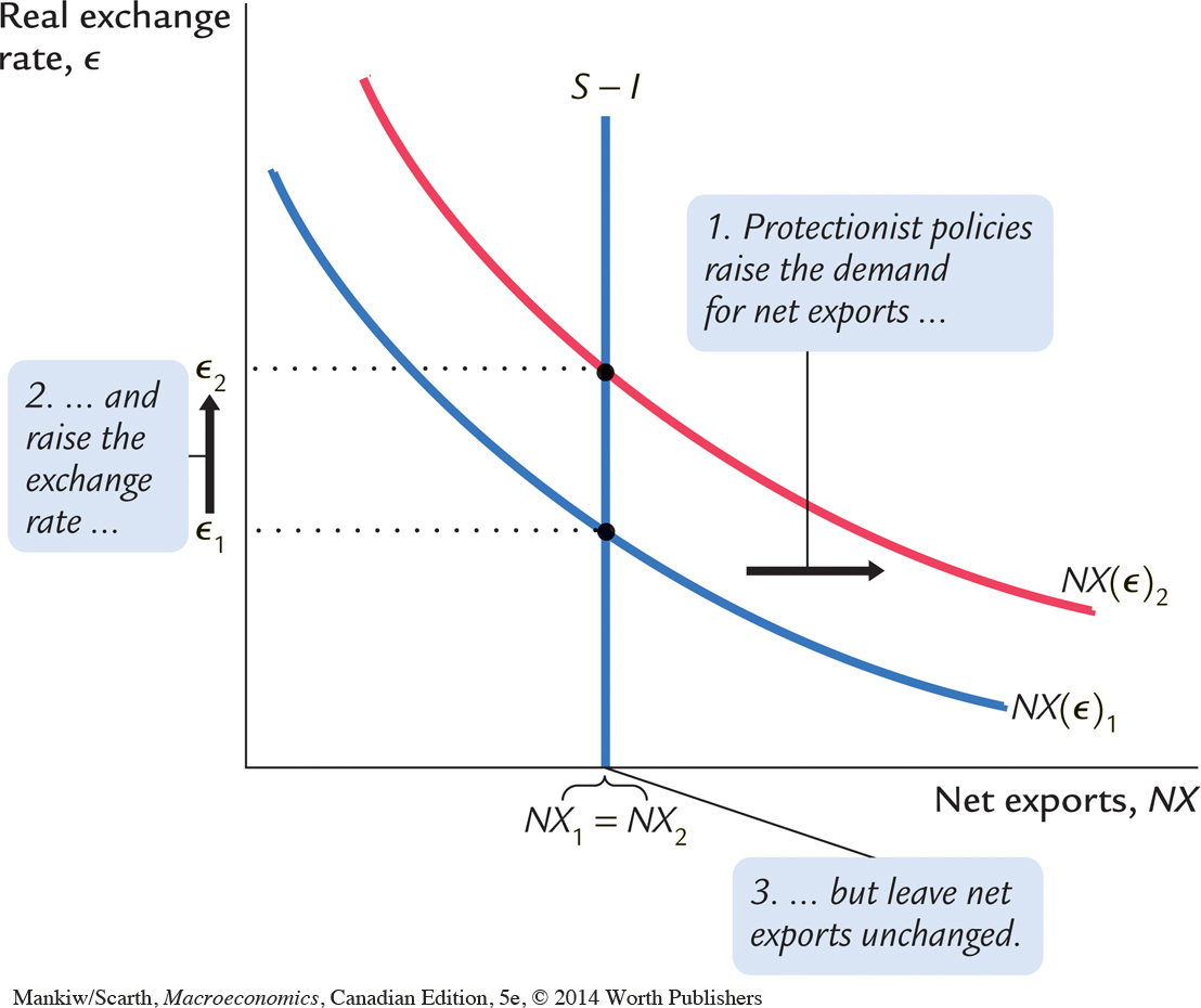
As an example of a protectionist trade policy, consider what would happen if the government prohibited the import of foreign cars. For any given real exchange rate, imports would now be lower, implying that net exports (exports minus imports) would be higher. Thus, the net-exports schedule shifts outward, as in Figure 5-13. To see the effects of the policy, we compare the old equilibrium and the new equilibrium. In the new equilibrium, the real exchange rate is higher, and net exports are unchanged. Despite the shift in the net-exports schedule, the equilibrium level of net exports remains the same, assuming the protectionist policy does not alter either saving or investment.
155
This analysis shows that protectionist trade policies do not affect the trade balance. This surprising conclusion is often overlooked in the popular debate over trade policies. Because a trade deficit reflects an excess of imports over exports, one might guess that reducing imports—such as by prohibiting the import of foreign cars—would reduce a trade deficit. Yet our model shows that protectionist policies lead only to an appreciation of the real exchange rate. The increase in the price of domestic goods relative to foreign goods tends to lower net exports by stimulating imports and depressing exports. Thus, the appreciation offsets the increase in net exports that is directly attributable to the trade restriction.
Although protectionist trade policies do not alter the trade balance, they do affect the amount of trade. As we have seen, because the real exchange rate appreciates, the goods and services we produce become more expensive relative to foreign goods and services. We therefore export less in the new equilibrium. Since net exports are unchanged, we must import less as well. (The appreciation of the exchange rate does stimulate imports to some extent, but this only partly offsets the decrease in imports due to the trade restriction.) Thus, protectionist policies reduce both the quantity of imports and the quantity of exports.
This fall in the total amount of trade is the reason economists almost always oppose protectionist policies. International trade benefits all countries by allowing each country to specialize in what it produces best and by providing each country with a greater variety of goods and services. Protectionist policies diminish these gains from trade. Although these policies benefit certain groups within society—for example, a ban on imported cars helps domestic car producers—society on average is worse off when policies reduce the amount of international trade.
CASE STUDY
The “Neo-Conservative” Policy Agenda in the 1980s and 1990s
During the 1984–1993 period, Canada’s Conservative government had an economic plan that involved four key elements:
Tax reform
Deficit reduction
Disinflation
Free trade
It is instructive to evaluate this package of initiatives using the analysis of this chapter.
The broad principle underlying tax reform was a move toward sales taxes and away from income taxes. This general move took several forms: (1) the introduction of the goods and services tax (GST), (2) the introduction of the capital gains tax exemption, and (3) the increase in the allowed contributions to registered retirement savings plans. All these initiatives were intended to stimulate private saving. Deficit reduction by the government itself is also a direct move toward higher national saving (since overall saving in the country is the excess of private saving over the government budget deficit). The reduction of inflation was also geared to stimulating saving, since (as we noted in Chapter 4) with nominal (not real) interest income subject to tax in Canada, lower inflation is equivalent to a cut in interest-income taxes.
156
Thus, the first three government initiatives were intended to shift the S − I line to the right, and so to lower the real exchange rate and increase the trade surplus. By increasing the rate at which Canadians become less indebted to foreigners, this policy package was intended to increase the standard of living for future generations.
The fourth policy initiative—free trade—has a less obvious effect on the trade balance. The Free Trade Agreement with the United States involved both countries dropping their tariffs by essentially the same amount. Thus, it involved at most a small net shift in the position of the net-exports schedule. But one of the expected outcomes was an increased level of investment spending in Canada. With access to the large U.S. market guaranteed (for firms located in Canada), it was expected that plants in Canada would expand. They no longer had to limit their operations to serve the small Canadian market. Such an increase in investment spending in Canada shifts the S − I line to the left. Thus, free trade involves competing effects on welfare: individuals can consume more goods at lower prices, but the investment effect that may accompany the removal of trade restrictions in the rest of the world leads to a larger trade deficit, and so (other things equal) to an increased level of foreign indebtedness in the future. The government was confident that the benefits would exceed the costs in this tradeoff for two reasons. First, the return on the extra capital employed in Canada should generate enough extra Canadian income for Canadians to be able to afford higher interest payments to foreigners. Second, the other three initiatives in the policy package were intended to increase domestic saving more than free trade increased investment. Thus, the net effect of the package was expected to be an increase in the trade surplus.
While this policy package can be rationalized easily within our analytical framework, it turned out that there were several slips between the design and the execution of these measures. First, the attempt to reduce the government’s budget failed; indeed, government deficits increased during this period. Second, changes to the tax system were only partial. The GST turned out to be an administrative headache, and it raised less revenue than was expected. Also, the capital gains exemption was reduced and then was eliminated in 1994. As a result, disinflation was the only policy (of the first three listed above) that was fully and successfully implemented while the Conservatives were in power. Thus, much of what was to shift the S − I line to the right did not materialize. As a result, the current account surplus did not rise appreciably. Unfortunately, for future generations of Canadians, the rate of foreign debt accumulation was not decreased appreciably.
157
This fact was not only a concern for future generations. Without the intended increase in national saving, the exchange rate remained higher in the late 1980s and early 1990s than had been the government’s intention. The high value of the Canadian dollar removed the competitive advantage that Canadian firms were getting through the reduction of U.S. tariffs. In the end, the fact that the government succeeded with respect to its monetary policy objective (disinflation) but failed with respect to its fiscal policy objective (deficit reduction) meant that the overall outcome for both current and future generations was far less than was possible given the basic consistency of the overall package of intended policies.
When the Liberals took power in the 1990s, they maintained the Conservative policy agenda. They made no further changes to the taxation of interest income and capital gains; they extended the Free Trade Agreement to include Mexico; and they maintained the low inflation policy. Since they contracted fiscal policy sufficiently to eliminate the budget deficit, national saving was increased and the current account surplus rose as a result. In the years that followed, Canadians enjoyed a lower level of indebtedness to foreigners.
The Determinants of the Nominal Exchange Rate
Having seen what determines the real exchange rate, we now turn our attention to the nominal exchange rate—the rate at which the currencies of two countries trade. Recall the relationship between the real and the nominal exchange rate:
Real Exchange Rate = Nominal Exchange Rate × Ratio of Price Levels
ϵ = e × (P/P*).
We can write the nominal exchange rate as
e = ϵ × (P*/P).
This equation shows that the nominal exchange rate depends on the real exchange rate and the price levels in the two countries. Given the value of the real exchange rate, if the domestic price level P rises, then the nominal exchange rate e will fall: because a dollar is worth less, a dollar will buy fewer yen. On the other hand, if the Japanese price level P* rises, then the nominal exchange rate will increase: because the yen is worth less, a dollar will buy more yen.
It is instructive to consider changes in exchange rates over time. The exchange rate equation can be written
% Change in e = % Change in ϵ + % Change in P* – % Change in P.
158
The percentage change in ϵ is the change in the real exchange rate. The percentage change in P is the domestic inflation rate π, and the percentage change in P* is the foreign country’s inflation rate π*. Thus, the percentage change in the nominal exchange rate is
% Change in e = % Change in ϵ + (π* – π)
Percentage Change in Nominal Exchange Rate = Percentage Change in Real Exchange Rate + Difference in Inflation Rates.
This equation states that the percentage change in the nominal exchange rate between the currencies of two countries equals the percentage change in the real exchange rate plus the difference in their inflation rates. If a country has a high rate of inflation relative to Canada, a Canadian dollar will buy an increasing amount of the foreign currency over time. If a country has a low rate of inflation relative to Canada, a Canadian dollar will buy a decreasing amount of the foreign currency over time.
This analysis shows how monetary policy affects the nominal exchange rate. We know from Chapter 4 that high growth in the money supply leads to high inflation. Here, we have just seen that one consequence of high inflation is a depreciating currency: high π implies falling e. In other words, just as growth in the amount of money raises the price of goods measured in terms of money, it also tends to raise the price of foreign currencies measured in terms of the domestic currency.
CASE STUDY
Inflation and Nominal Exchange Rates
If we look at data on exchange rates and price levels of different countries, we quickly see the importance of inflation for explaining changes in the nominal exchange rate. The most dramatic examples come from periods of very high inflation. For example, the price level in Mexico rose by 2,300 percent from 1983 to 1988. Because of this inflation, the number of pesos a person could buy with a U.S. dollar rose from 144 in 1983 to 2,281 in 1988.
The same relationship holds true for countries with more moderate inflation. Figure 5-14 is a scatterplot showing the relationship between inflation and the exchange rate for 15 countries. On the horizontal axis is the difference between each country’s average inflation rate and the average inflation rate of the United States, our base for comparison. This is our measure of (π* – π). On the vertical axis is the average percentage change in the exchange rate between each country’s currency and the U.S. dollar (% Change in e). The positive relationship between these two variables is clear in this figure. Countries with relatively high inflation tend to have depreciating currencies, and countries with relatively low inflation tend to have appreciating currencies.
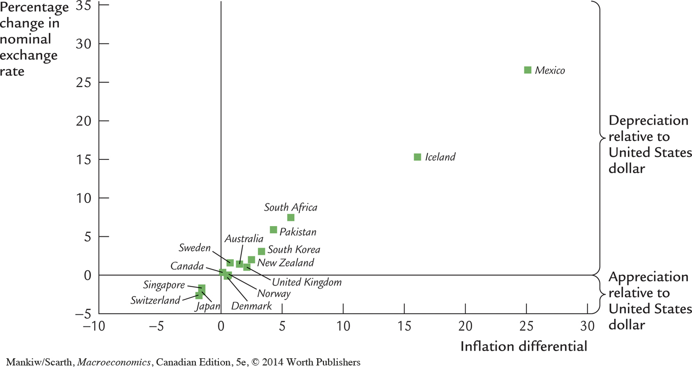
As an example, consider the exchange rate between Swiss francs and U.S. dollars. Both Switzerland and the United States have experienced inflation over the past twenty years, so both the franc and the dollar buy fewer goods than they once did. But, as Figure 5-14 shows, inflation in Switzerland has been lower than inflation in the United States. This means that the value of the franc has fallen less than the value of the dollar. Therefore, the number of Swiss francs one can buy with a U.S. dollar has been falling over time.
The Special Case of Purchasing-Power Parity
159
A famous hypothesis in economics, called the law of one price, states that the same good cannot sell for different prices in different locations at the same time. If a tonne of wheat sold for less in Calgary than in Winnipeg, it would be profitable to buy wheat in Calgary and then sell it in Winnipeg. This profit opportunity would become quickly apparent to astute arbitrageurs—people who specialize in “buying low” in one market and “selling high” in another. As the arbitrageurs took advantage of this opportunity, they would increase the demand for wheat in Calgary and increase the supply in Winnipeg. This would drive the price up in Calgary and down in Winnipeg—thereby ensuring that prices are equalized in the two markets.
160
The law of one price applied to the international marketplace is called purchasing-power parity. It states that if international arbitrage is possible, then a dollar (or any other currency) must have the same purchasing power in every country. The argument goes as follows. If a dollar could buy more wheat domestically than abroad, there would be opportunities to profit by buying wheat domestically and selling it abroad. Profit-seeking arbitrageurs would drive up the domestic price of wheat relative to the foreign price. Similarly, if a dollar could buy more wheat abroad than domestically, the arbitrageurs would buy wheat abroad and sell it domestically, driving down the domestic price relative to the foreign price. Thus, profit-seeking by international arbitrageurs causes wheat prices to be the same in all countries.
We can interpret the doctrine of purchasing-power parity using our model of the real exchange rate. The quick action of these international arbitrageurs implies that net exports are highly sensitive to small movements in the real exchange rate. A small decrease in the price of domestic goods relative to foreign goods—that is, a small decrease in the real exchange rate—causes arbitrageurs to buy goods domestically and sell them abroad. Similarly, a small increase in the relative price of domestic goods causes arbitrageurs to import goods from abroad. Therefore, as in Figure 5-15, the net-exports schedule is very flat at the real exchange rate that equalizes purchasing power among countries: any small movement in the real exchange rate leads to a large change in net exports. This extreme sensitivity of net exports guarantees that the equilibrium real exchange rate is always close to the level that ensures purchasing-power parity.
Purchasing-power parity has two important implications. First, since the net-exports schedule is flat, changes in saving or investment do not influence the real or nominal exchange rate. Second, since the real exchange rate is fixed, all changes in the nominal exchange rate result from changes in price levels.
Is this doctrine of purchasing-power parity realistic? Most economists believe that, despite its appealing logic, purchasing-power parity does not provide a completely accurate description of the world. First, many goods are not easily traded. A haircut can be more expensive in Tokyo than in Toronto, yet there is no room for international arbitrage since it is impossible to transport haircuts. Second, even tradeable goods are not always perfect substitutes. Some consumers prefer Toyotas, and others prefer Fords. Thus, the relative price of Toyotas and Fords can vary to some extent without leaving any profit opportunities. For these reasons, real exchange rates do in fact vary over time.
161
Although the doctrine of purchasing-power parity does not describe the world perfectly, it does provide a reason why movement in the real exchange rate will be limited. There is much validity to its underlying logic: the farther the real exchange rate drifts from the level predicted by purchasing-power parity, the greater the incentive for individuals to engage in international arbitrage in goods. Although we cannot rely on purchasing-power parity to eliminate all changes in the real exchange rate, this doctrine does provide a reason to expect that a significant number of the changes in the real exchange rate may be temporary.3
CASE STUDY
The Big Mac Around the World
The doctrine of purchasing-power parity says that after we adjust for exchange rates, we should find that goods sell for the same price everywhere. Conversely, it says that the exchange rate between two currencies should depend on the price levels in the two countries.
To see how well this doctrine works, The Economist, an international newsmagazine, regularly collects data on the price of a good sold in many countries: the McDonald’s Big Mac hamburger. According to purchasing-power parity, the price of a Big Mac should be closely related to the country’s nominal exchange rate. The higher the price of a Big Mac in the local currency, the higher the exchange rate (measured in units of local currency per U.S. dollar) should be.
Table 5-2 presents the international prices in 2011, when a Big Mac sold for $4.07 in the United States (this was the average price in New York, San Francisco, Chicago, and Atlanta). With these data we can use the doctrine of purchasing-power parity to predict nominal exchange rates. For example, because a Big Mac cost 320 yen in Japan, we would predict that the exchange rate between the dollar and the yen was 320/4.07, or around 78.6 yen per dollar. At this exchange rate, a Big Mac would have cost the same in Japan and the United States.
| Exchange Rate (per U.S. dollar) | ||||
| Country | Currency | Price of a Big Mac | Predicted | Actual |
| Indonesia | Rupiah | 22534.00 | 5537 | 8523.0 |
| Colombia | Peso | 8400.00 | 2064 | 1771.0 |
| South Korea | Won | 3700.00 | 909 | 1056.0 |
| Chile | Peso | 1850.00 | 455 | 463.0 |
| Hungary | Forint | 760.00 | 187 | 188.0 |
| Japan | Yen | 320.00 | 78.6 | 78.4 |
| Pakistan | Rupee | 205.00 | 50.4 | 86.3 |
| Philippines | Peso | 118.00 | 29.0 | 42.0 |
| India | Rupee | 84.00 | 20.6 | 44.4 |
| Russia | Rouble | 75.00 | 18.4 | 27.8 |
| Taiwan | NT Dollar | 75.00 | 18.4 | 28.8 |
| Thailand | Baht | 70.00 | 17.2 | 29.8 |
| Czech Republic | Koruna | 69.30 | 17.0 | 17.0 |
| Sweden | Krona | 48.40 | 11.9 | 6.3 |
| Norway | Kroner | 45.00 | 11.1 | 5.4 |
| Mexico | Peso | 32.00 | 7.86 | 11.70 |
| Denmark | D. Krone | 28.50 | 7.00 | 5.20 |
| Argentina | Peso | 20.00 | 4.91 | 4.13 |
| South Africa | Rand | 19.45 | 4.78 | 6.77 |
| Israel | Shekel | 15.90 | 3.91 | 3.40 |
| Hong Kong | HK Dollar | 15.10 | 3.71 | 7.79 |
| China | Yuan | 14.70 | 3.61 | 6.45 |
| Egypt | Pound | 14.10 | 3.46 | 5.96 |
| Peru | Sol | 10.00 | 2.46 | 2.74 |
| Saudi Arabia | Riyal | 10.00 | 2.46 | 3.75 |
| Brazil | Real | 9.50 | 2.33 | 1.54 |
| Poland | Zloty | 8.63 | 2.12 | 2.80 |
| Malaysia | Ringgit | 7.20 | 1.77 | 2.97 |
| Switzerland | S. Franc | 6.50 | 1.60 | 0.81 |
| Turkey | Lira | 6.50 | 1.60 | 1.72 |
| New Zealand | NZ Dollar | 5.10 | 1.25 | 1.16 |
| Canada | C. Dollar | 4.73 | 1.16 | 0.95 |
| Australia | A. Dollar | 4.56 | 1.12 | 0.92 |
| Singapore | S. Dollar | 4.41 | 1.08 | 1.21 |
| United States | Dollar | 4.07 | 1.00 | 1.00 |
| Euro area | Euro | 3.44 | 0.85 | 0.70 |
| Britain | Pound | 2.39 | 0.59 | 0.61 |
|
Note: The predicted exchange rate is the exchange rate that would make the price of a Big Mac in that country equal to its price in the United States. Source: The Economist, July 28, 2011. |
||||
|---|---|---|---|---|
Table 5-2 shows the predicted and actual exchange rates for 36 countries plus the Euro area, ranked by the predicted exchange rate. You can see that the evidence on purchasing-power parity is mixed. As the last two columns show, the actual and predicted exchange rates are usually in the same ballpark. Our theory predicts, for instance, that a U.S. dollar should buy the greatest number of Indonesian rupiahs and fewest British pounds, and this turns out to be true. In the case of Japan, the predicted exchange rate of 78.6 yen per dollar is very close to the actual exchange rate of 78.4. Yet the theory’s predictions are far from exact and in many cases are off by 30 percent or more. Hence, although the theory of purchasing-power parity provides a rough guide to the level of exchange rates, it does not explain exchange rates completely. Part of the explanation for this incomplete matching between theory and evidence is surely related to the fact that arbitrage is difficult with a perishable commodity such as a hamburger.
162