206

APPENDIX

Unemployment, Inequality, and Government Policy

The efficiency-wage model is one theory of unemployment that was discussed in the main body of this chapter. In this appendix, we describe a specific version of this model that can be used as a vehicle to assess some common presumptions—such as “payroll taxes are job killers” and “globalization makes rising income inequality inevitable.”

As explained earlier, one common version of the efficiency-wage model is based on the assumption of asymmetric information. Employees know whether they are shirking, but employers cannot be sure. To mention just one consideration, it is impossible for employers to verify fully whether individual employees can be believed when they call in sick. Firms can lessen this worker-productivity problem by making it more expensive for employees to lose their jobs. By paying a wage that exceeds each worker’s alternative option, employers can ensure that their employees work hard to avoid being fired. But when all firms raise payments in this way, the overall level of wages exceeds what would obtain in a competitive market. With labour more expensive, firms hire fewer workers in total, and there is unemployment, as shown in Figure 6-3.

It is worthwhile formalizing this model of the labour market. Let w and b stand for the wage a worker receives from her employer and the income she can expect if she leaves that firm, respectively. With the firm’s incomplete monitoring process, there is a probability that the worker can be fired for low productivity. That probability can be reduced by putting forth more effort, but this effort decreases the utility that the employee receives while at work. Let fraction a times the wage represent the income equivalent of the loss in utility that stems from this extra effort.

The worker faces two options: either she stays on the job with a net return of (1 - a)w, or she is fired, in which case she receives b. Firms will get high productivity from workers as long as (1 -–a)w is greater than or equal to b. But in the interest of minimizing wage costs, firms do not want to meet this constraint with any unnecessary payment, so they set

w = b/(1 - a).

Since a is a fraction, this equation verifies that firms set wages above the workers’ alternative.

How is b, the workers’ alternative, determined? Again, there are two options. A fired worker may get employed by another firm (and the probability of this outcome is the economy’s employment rate, (1 -–u)), or she may go without work (and the probability of this happening is the unemployment rate, u). In a full equilibrium, all firms have to pay the same wage to keep their workers. Finally, for simplicity, let us assume that there is an employment-insurance program that pays workers fraction c of their former wage if they are out of work. All this means that each worker’s alternative is

207

b = (1 – u)w + u(cw).

When this definition of the alternative option is substituted into the wage-setting rule, w = b/(1 - a), the result can be simplified to

u = a/(1 – c).

This expression for the full-equilibrium structural unemployment rate indicates three things. First, if workers do not find hard work distasteful at all (that is, if a = 0), firms would not need to set wages above the competitive level to limit any shirking problem, so there would be no unemployment. (Implicitly, this is what we assumed in Chapter 3.) Second, since there is no variable relating to worker skill or education levels in the unemployment-rate equation, changes in these factors do not affect employment. If workers are more skilled, both their current employer and other potential employers are prepared to pay them more. So wages rise generally and there are no changes in the incentive to shirk. The model is consistent with experience in this regard. Labour productivity increased dramatically over the twentieth century and, just as the model predicts, we observed a vast increase in real wages and no long-term trend in the unemployment rate.

The third implication of this model is that the unemployment problem is accentuated by a more generous employment-insurance program (a higher value for c). The reason? More generous support for unemployment lowers the cost of being fired. Workers react by shirking more, so firms react by raising wages. With higher wages, firms find it profitable to hire fewer workers. Since unemployment insurance is a form of income redistribution, the model illustrates the standard tradeoff involved: the size of the overall economic pie shrinks when we try to redistribute. This fact does not mean that redistribution should be rejected. Society may prefer a higher unemployment rate if each individual involved is better protected from hardship.

Let us extend this model to allow for payroll and personal income taxes. Employees pay tax rate t times their wages, while employment-insurance receipts are not taxed. Since workers keep only proportion (1 - t) of each dollar earned on the job, the revised expressions are w(1 – t)(1 – a) = b and b = (1 – u)w(1 – t) +u(cw). These relationships lead to a revised expression for the steady-state unemployment rate:

u = a(1 – t)/(1 – c – t).

We see that the unemployment rate depends on the tax rate faced by employees. Higher taxes lower the return from working. To counteract the resulting increased propensity to shirk, firms raise wages and fewer individuals find jobs.

An important insight can be gained by inserting representative numerical values for each term in the unemployment-rate equation. Initially, let us assume a tax rate of 15 percent (t = 0.15), an employment insurance program that pays each former worker one-half of what she previously earned (c = 0.5), and a shirking parameter value (a = 0.02) that yields a representative value for unemployment of 5 percent (u = 0.05). Now we investigate how much the unemployment rate rises as we consider higher values for the tax rate (and the other parameters, c and a, are fixed). You can verify that as the tax rate rises by equal amounts, first from 15 to 25 percent and then from 25 to 35 percent, the unemployment rate rises, first by 1 percentage point, from 5 to 6 percent, and then by 2.67 percentage points, from 6 to 8.67 percent. Clearly, the unemployment rate rises much more when taxes are already high. The model is consistent with the widespread drive to lower taxes.

208

It is noteworthy that the employer payroll tax rate does not affect unemployment. Just like an increase in general productivity, a lower employer payroll tax rate raises both the firms’ willingness to pay higher wages and the workers’ wage claims. As a result, unemployment can be reduced by a revenue-neutral cut in the employee payroll tax rate (financed by an increase in the employer payroll tax rate).

The major payroll taxes in Canada are the contributions to employment insurance (EI) and to the public pension programs (the CPP and QPP). During the late 1990s, the contributions to EI were reduced by a small amount each year (because the EI account was in surplus), but the contributions to the CPP/QPP were increased a great deal more (because this is how the government chose to keep the public pension system from going bankrupt as the baby-boom generation ages). Since, on balance, payroll taxes have risen, there has been upward pressure on unemployment. It is unfortunate that the government has not decreased its reliance on the employee portion of this levy, since (as this model illustrates) such a change in policy could reverse this upward pressure on the unemployment rate.

Many people fear that globalization is leading to higher unemployment. Compared to many low-wage countries, Canada has an abundance of skilled workers and a relatively small proportion of the population in the unskilled category. The opposite is the case in the developing countries. With increased integration among the world economies, Canada specializes in the production of goods that emphasize our relatively abundant factor, skilled labour, so it is the wages of skilled workers that are bid up by increased foreign trade. The other side of this development is that Canada relies more on imports to supply goods that only require unskilled labour, and this means that the demand for unskilled labour falls in Canada. The result is either lower wages for the unskilled in Canada (if there is no legislation that puts a floor on wages here) or rising unemployment among the unskilled (if there is a floor on wages—such as that imposed by minimum-wage laws). In either case, unskilled individuals can lose in the new global economy.

As noted in the main text of this chapter, a second hypothesis concerning rising income inequality is that, during the last several decades, technological change has been decidedly skill-biased—with the result that the demand for skilled workers has risen while that for the unskilled has fallen. Just as with the globalization hypothesis, the effects of these shifts in demand depend on whether it is possible for wages in the unskilled sector to fall. The United States and Europe are often cited as illustrations of the possible outcomes. The United States has only a limited welfare state, so there is little to stop increased wage inequality from emerging, as indeed it has in recent decades. European governments, on the other hand, maintain floors below which the wages of the unskilled cannot be pushed. When technological change decreases the demand for unskilled labour, firms have no freedom to do anything but reduce their employment of these individuals. Thus, Europe has avoided large increases in wage inequality, but the unemployment rate has been very high there for many years.

209

Most economists favour the second hypothesis for explaining rising income inequality. This is because inequality has increased so much within each industry and occupation, in ways that are unrelated to foreign trade. But whatever the cause, the plight of the less skilled is a dire one. Figure 6-6 allows us to consider policy options.

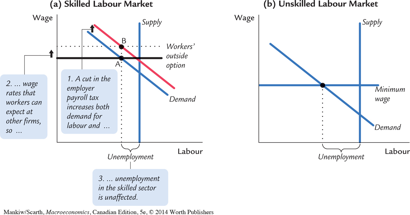
Panel (a) in Figure 6-6 depicts the skilled labour market, while panel (b) illustrates the unskilled market. There is unemployment in both sectors. In the skilled labour market, unemployment is due to incomplete information and efficiency wages. In the unskilled market, unemployment is due to minimum wages. Let us consider a reduction in employer payroll taxes. Cutting the tax that employers must pay when hiring skilled workers results in a shift up in the demand for skilled labour. But since all firms react in this same way, the workers’ outside option rises to the same extent, so the market outcome moves from a point A to point B in panel (a) of Figure 6-6. No jobs are created. Indeed, some jobs may be destroyed. If the value of the minimum wage is set as some fixed proportion of wages in the skilled sector, there is one further effect. The minimum-wage line shifts up in panel (b) of the figure, and unemployment among the unskilled is higher. So this model does not support cutting the employer payroll tax associated with skilled workers.

210

Cutting the tax that employers must pay when hiring unskilled workers results in an upward shift in the demand for unskilled labour. Since the position of no other curve in either market is affected by this policy, it is obvious—without our showing it in panel (b)—that this initiative reduces unemployment in the unskilled sector. Thus, the elimination of payroll taxes levied on employers for hiring unskilled workers is supported by the model. Indeed, offering employment subsidies (a negative employer payroll tax) for (only) low-wage workers has been recommended by all leading economists who have addressed the issue of rising income inequality.

This proposal respects the proposition that lasting jobs are best generated through the private sector, and that market failure is a precondition for governments to adjust market signals. It has been shown²¹ that even revenue-neutral versions of this initiative generate favourable spillover outcomes—higher wages for skilled workers and higher investment—in addition to lower unemployment for the less skilled. In contrast to “trickle-down” measures (which involve direct benefits for the well-to-do and indirect benefits for others), the low-wage subsidy is a “percolate-up” strategy (which confers direct benefits for the less well-to-do and indirect benefits for others). Trickle-down economics was considered in the appendix to Chapter 5.

Our discussion of policies that can lower the natural unemployment rate raises a general issue that has been much in the news in recent years. Every time there is a meeting of country representatives to such organizations as the International Monetary Fund or the World Bank, there is a major demonstration in the streets by antiglobalization protesters. These individuals resent the fact that the “neoconservative” world bodies focus on keeping capital free to move between countries. These institutions favour capital mobility on the grounds that world incomes will be maximized only if capital is free to locate where it has the highest marginal product. But the protesters are more concerned with the position of labourers, not capital owners. They want labour’s income—not overall income—to be higher.

211

The antiglobalization protesters focus on the following concern: how can the government in a small open economy provide low-income support policies for its citizens? We can address this issue by thinking of labour as the low-income or “poor” individuals and by thinking of capital owners as the “rich.” If the government is to make transfers payments to the “poor,” they must raise the necessary revenue by trying to tax the “rich.” But if the rich can costlessly transfer their capital to be employed in low-tax countries, our government will not be able to make the tax stick on capitalists. It would seem that there is no way to help the economic position of labour if capital cannot be taxed. The protesters’ answer to this problem is to restrict the mobility of capital (that is, to limit globalization). But there is another way out of the dilemma.

We use Figure 6-7 to analyze the options available to the government. This analysis is similar to the discussion on trickle-down economics in the appendix to Chapter 5. So if you find that you do not understand the present analysis fully, review the material in the previous chapter. In panel (a) of Figure 6-7, we see a picture of the economy’s capital market. Since it is profit-maximizing for firms to hire capital as long as its marginal product exceeds the rent that must be paid, the downward-sloping marginal product relationship is the demand curve for capital. The perfectly elastic supply curve indicates that the owners of capital will supply capital to this economy in unlimited amounts if they receive the return that is available in the rest of the world. This means that capital is withdrawn from this economy if the after-tax return is at all below the yield available elsewhere. The fact that this supply curve is horizontal is the globalization constraint that the domestic policymaker must contend with.

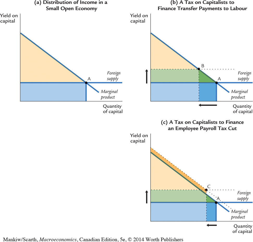
With no tax on the owners of capital, the economy is observed at point A—the intersection of supply and demand. Since the area under the marginal product curve represents total product, the country’s GDP is given by the coloured trapazoid in panel (a). Capitalists receive a total income equal to the light blue rectangle, and labour receives the rest of national income—the light beige triangle. We are assuming that the government wants to increase what labour gets. If the government levies a tax on the earnings of capital, the owners react by demanding a higher pretax return. Indeed, if the pretax return does not rise by just enough to leave the after-tax yield equal to what is available elsewhere, then capitalists will withdraw from this country. Geometrically, we impose this reaction by shifting the capital supply curve up by just the amount of the tax [as shown in panel (b)]. The intersection of the now relevant supply and demand curves is at point B. By comparing the before-tax and after-tax outcome points (A and B), we see that some capital has left the country. As a result, the GDP is smaller; with the tax it is just the sum of the light-beige, light-green, and light-blue areas.

Not all the capital leaves the country. Once some units have left, what remains is more scarce, so it has a higher marginal product—just enough to generate a payment that covers the tax obligation. The capital that remains gets after-tax income equal to the light blue area, exactly what it received before the tax. The capital that leaves the country receives the dark blue area (elsewhere), exactly what it used to receive here. So capitalists are totally unaffected by the tax. This is the globalization constraint.

212

The government collects tax revenue equal to the light green rectangle. Since this comes out of the triangle that labour used to receive before the tax, it is labour that truly bears the burden of the tax. But since the whole point of levying the tax is to make a transfer payment to labour, this group both pays out and gets back the light green area. So labour is neither helped nor hurt by the transfers. But labour is worse off on balance because there is still the loss of the dark green triangle (that used to be—but is no longer—part of labour’s receipts). This loss exists because labour has less capital to work with. This makes workers less productive, and lower productivity leads to lower wages. So this standard supply-demand analysis supports the concern of the antiglobalization protesters. It appears that the attempt to help the “poor” has failed; indeed, they are worse off after the government’s attempt to help them!

213

But before you get too excited about joining the protesters in the streets, consider the fact that our analysis has so far involved the assumption that the government intervention has had no effect on the natural unemployment rate. As we learned earlier in this appendix, the unemployment rate can be lowered if the government uses the revenue to cut the employee payroll tax. Panel (c) in Figure 6-7 shows how the analysis is altered when the government does use the revenue in this way, rather than by making a straight transfer payment to labour.

As before, a tax that is intended to be borne by capitalists is levied to give the government the necessary revenue to finance the payroll tax cut. Thus, the supply curve shifts up by the amount of the tax in panel (c). But with the payroll tax cut leading to lower unemployment, capital now has more labour to work with, and this increases capital’s productivity. We show this in the diagram by shifting capital’s marginal product curve out to the right. The intersection of the now relevant supply and demand curves is at point C. Comparing the locations of outcome points B and C, we can appreciate that less capital leaves the country when the policy package involves a reduction in unemployment. This means that labour’s net loss in the previous scenario—the dark green triangle—is now smaller in panel (c). And this is not the only piece of good news. There is an area indicating a gain in the size of labour’s triangle—the dark beige band in panel (c). This region represents the additional output that was not being produced before, when more individuals were out of work.

It is too messy to show here, but labour’s gain (the dark beige band) is almost certainly bigger than labour’s loss (the dark green triangle). Specifically, we can combine a Cobb–Douglas production function and the efficiency-wage model of unemployment discussed earlier in the appendix. If the analysis is repeated in an algebraic mode (with these components), it can be shown that this tax substitution (a higher tax on capital combined with a lower payroll tax) must lead to an improvement in labour’s position.

So the antiglobalization protesters have been premature in reaching the view that governments are unable to provide low-income support policy in a globalized setting. Our analysis supports their contention that the government cannot make taxes stick on the capitalists. This means that redistribution—taking from the rich and giving to the poor—is not possible. But as we have seen, there is another way to help the poor. Instead of trying to redistribute income, the government can simply decrease wastage by reducing structural unemployment. This increases the overall size of the economic pie, so that the poor can get a bigger slice without our having to reduce the size of the slice that the rich receive. The moral of the story is that the provision of low-income support in a globalized setting requires that the government focus on initiatives that can be expected to reduce structural unemployment. As a result, the analysis in this chapter is central to the challenges that will face Canada’s policymakers in the coming years.

214

It should now be clearer why economists are applauding Canadian policymakers for introducing the Working Income Tax Benefit, rather than relying exclusively on standard welfare programs and employment insurance. Transfers to those on lower incomes can be made in three broad ways. First, the transfer can be conditional on the individual being unemployed (as in EI). This transfer has the unfortunate side effect of raising unemployment. The second option is welfare in the form of a guaranteed annual income. This policy involves a low-income transfer that is independent of an individual’s employment status, so it does not have the unfortunate side effect of raising unemployment. The third option is some form of low-income employment subsidy (a negative payroll tax). This transfer payment only goes to those who are working, so the side effect in this case is a desirable one—a lower unemployment rate.