270

A chemist, a physicist, and an economist are all trapped on a desert island, trying to figure out how to open a can of food.

“Let’s heat the can over the fire until it explodes,” says the physicist.

“No, no,” says the engineer, “Let’s drop the can onto the rocks from the top of a high tree.”

“I have an idea,” says the economist. “First, we assume a can opener . . . .”

This old joke takes aim at how economists use assumptions to simplify—and sometimes oversimplify—the problems they face. It is particularly apt when evaluating the theory of economic growth. One goal of growth theory is to explain the persistent rise in living standards that we observe in most parts of the world. The Solow growth model shows that such persistent growth must come from technological progress. But where does technological progress come from? In the Solow model, it is just assumed!

The preceding Case Study on the productivity slowdown of the 1970s and speedup of the 1990s suggests that changes in the pace of technological progress are tremendously important. To understand fully the process of economic growth, we need to go beyond the Solow model and develop models that explain technological advance. Models that do this often go by the label endogenous growth theory because they reject the Solow model’s assumption of exogenous technological change. Although the field of endogenous growth theory is large and sometimes complex, here we get a quick taste of this modern research.¹³

To illustrate the idea behind endogenous growth theory, let’s start with a particularly simple production function:

Y = AK,

where Y is output, K is the capital stock, and A is a constant measuring the amount of output produced for each unit of capital. Notice that this production function does not exhibit the property of diminishing returns to capital. One extra unit of capital produces A extra units of output, regardless of how much capital there is. This absence of diminishing returns to capital is the key difference between this model and the Solow model.

271

Now let’s see what this production function says about economic growth. As before, we assume a fraction s of income is saved and invested. We therefore describe capital accumulation with an equation similar to those we used previously:

ΔK = sY – δK.

This equation states that the change in the capital stock (ΔK) equals investment (sY) minus depreciation (δK). (For simplicity in this derivation, we abstract from population growth.) Combining this equation with the Y = AK. production function, we obtain after a bit of manipulation

ΔY/Y = ΔK/K = sA – δ.

This equation shows what determines the growth rate of output ΔY/Y. Notice that, as long as sA > δ, the economy’s income grows forever, even without the assumption of exogenous technological progress.

Thus, a simple change in the production function can alter dramatically the predictions about economic growth. In the Solow model, saving leads to growth temporarily, but diminishing returns to capital eventually force the economy to approach a steady state in which growth depends only on exogenous technological progress. By contrast, in this endogenous growth model, saving and investment can lead to persistent growth.

But is it reasonable to abandon the assumption of diminishing returns to capital? The answer depends on how we interpret the variable K in the production function Y = AK. If we take the traditional view that K includes only the economy’s stock of plants and equipment, then it is natural to assume diminishing returns. Giving 10 computers to a worker does not make that worker ten times as productive as he or she is with one computer.

Advocates of endogenous growth theory, however, argue that the assumption of constant (rather than diminishing) returns to capital is more palatable if K is interpreted more broadly. Earlier in this chapter, we interpreted K as only physical capital, and the level of knowledge was part of what was incorporated into the efficiency of labour parameter E. Here we are suggesting an alternative interpretation. Perhaps the best case for the endogenous growth model is to view knowledge as a type of capital. Clearly, knowledge is an important input into the economy’s production—both its production of goods and services and its production of new knowledge. Compared to other forms of capital, however, it is less natural to assume that knowledge exhibits the property of diminishing returns. (Indeed, the increasing pace of scientific and technological innovation over the past few centuries has led some economists to argue that there are increasing returns to knowledge.) If we accept the view that knowledge is a type of capital, then this endogenous growth model with its assumption of constant returns to capital becomes a more plausible description of long-run economic growth.

The policy implications of this basic endogenous growth model are worth illustrating quantitatively. To do so, however, we need to rely on the more advanced theory of household consumption behaviour covered in Section 17-2. As a result, readers may wish to reread the remainder of this subsection after covering Chapter 17, but it is worth skim-reading this material at this stage, because the general idea can still be appreciated.

272

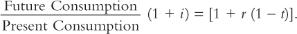
We learn in Chapter 17 that forward-looking households optimize by setting the marginal rate of substitution between current and future consumption equal to the ratio of the prices of present and future consumption. Since postponing consumption allows the household to earn the after-tax interest rate, r(1 – t), on those funds, the household has more resources if it waits to consume in the future. Thus, the present-to-future price ratio equals [1 + r (1 – t)]. The marginal rate of substitution is the ratio of current marginal utility to future marginal utility. The simplest function that involves diminishing marginal utility of consumption at each point in time and impatience across time is

where i is the household’s rate of impatience. For this utility function, current marginal utility is (1/Present Consumption) and future marginal utility is (1/Future Consumption)[1/(1 + i)]. Equating the resulting expression for the marginal rate of substitution to the price ratio, we have

We can simplify this optimal consumption rule by moving the (1 + i) term to the denominator on the right-hand side, by subtracting one from both sides, and by denoting present and future consumption by C₁ and C₂ respectively. The result is

(C₂ – C₁)/C₁ = (1 + r (1 – t) – 1 – i)/(1 + i).

For any reasonable value for the annual rate of impatience, such as 0.04, the value of (1 + i) is very close to unity, so we can make this approximation. With this simplification, the optimal purchase rule amounts to saying that—to optimize—households must arrange their affairs so that the percentage growth in consumption equals the excess of the after-tax interest they receive on their saving over their rate of impatience. Using the symbols we have used in this chapter to represent the growth rate of income and consumption, n + g, we have

n + g = Growth Rate = r (1 – t) – i.

We now use this relationship to illustrate how much government policy can affect the growth rate.

In the Y = AK model, the marginal product of capital r is a constant A. The household’s rate of impatience i is also independent of fiscal policy. Thus, the government’s tax rate is the only variable on the right-hand side of the equation that changes. For an illustration of the effect of tax policy on the growth rate, let us assume that capital’s marginal product is 8 percent, the household rate of impatience is 4 percent, and the tax rate is 25 percent (r = 0.08, i = 0.04, t = 0.25). These assumptions make the growth rate 2 percent (n + g = 0.02). Now consider the tax rate being reduced by just two percentage points (to 0.23). The right-hand side of our growth-rate equation rises by r times 0.02, or by 0.0016. We conclude that the annual growth rate for consumption rises by about one-sixth of one percentage point. Is this a significant increase? It doesn’t seem like much, but it represents more consumption for households—every year forever. We now calculate the present value of this ongoing series of small improvements in living standards.

273

Let us choose units so that present consumption is unity. The present value of all present and future consumption is then one divided by the excess of the household’s rate of impatience over the rate at which consumption is growing: 1/[i – (n + g)]. Initially, before the tax cut, this expression equals 1/(0.04 – 0.02) = 50. After the tax cut, this expression equals 1/(0.04 – 0.0216) = 54.3. So a small cut in the tax rate—just two percentage points—raises consumption by a one-time equivalent amount that is four and one-third times as big as an entire year’s consumption! That represents a lot of hospitals, day care centres, and social benefits.

We conclude that the basic endogenous growth model has a very exciting property. It suggests that even small tax changes—ones that are well within the range of what can be executed from a political point of view—can have rather dramatic effects on material living standards. This explains Robert Lucas’s expression of excitement in the quotation that starts this chapter and explains why macroeconomists have devoted a lot of research effort to investigating whether such results are found in more elaborate versions of endogenous growth theory.

Although the Y = AK model is the simplest example of endogenous growth, the theory has gone well beyond this. One line of research has tried to develop models with more than one sector of production in order to offer a better description of the forces that govern technological progress. To see what we might learn from such models, let’s sketch out an example.

The economy has two sectors, which we can call manufacturing firms and research universities. Firms produce goods and services, which are used for consumption and investment in physical capital. Universities produce a factor of production called “knowledge,” which is then freely used in both sectors. The economy is described by the production function for firms, the production function for universities, and the capital-accumulation equation:

Y = F[K,(1 – u)LE] (production function in manufacturing firms),

ΔE = g(u)E(production function in research universities),

ΔK = sY – δK(capital accumulation),

where u is the fraction of the labour force in universities (and 1 – u is the fraction in manufacturing), E is the stock of knowledge (which in turn determines the efficiency of labour), and g is a function that shows how the growth in knowledge depends on the fraction of the labour force in universities. The rest of the notation is standard. As usual, the production function for the manufacturing firms is assumed to have constant returns to scale: if we double both the amount of physical capital (K) and the number of effective workers in manufacturing [(1 – u)EL], we double the output of goods and services (Y).

274

This model is a cousin of the Y = AK model. Most important, this economy exhibits constant (rather than diminishing) returns to capital, as long as capital is broadly defined to include knowledge. In particular, if we double both physical capital K and knowledge E, then we double the output of both sectors in the economy. As a result, like the Y – AK model, this model can generate persistent growth without the assumption of exogenous shifts in the production function. Here persistent growth arises endogenously because the creation of knowledge in universities never slows down.

At the same time, however, this model is also a cousin of the Solow growth model. If u, the fraction of the labour force in universities, is held constant, then the efficiency of labour E grows at the constant rate g(u). This result of constant growth in the efficiency of labour at rate g is precisely the assumption made in the Solow model with technological progress. Moreover, the rest of the model—the manufacturing production function and the capital-accumulation equation—also resembles the rest of the Solow model. As a result, for any given value of u, this endogenous growth model works just like the Solow model.

There are two key decision variables in this model. As in the Solow model, the fraction of output used for saving and investment, s, determines the steady-state stock of physical capital. In addition, the fraction of labour in universities, u, determines the growth in the stock of knowledge. Both s and u affect the level of income, although only u affects the steady-state growth rate of income. Thus, this model of endogenous growth takes a small step in the direction of showing which societal decisions determine the rate of technological change.

The two-sector endogenous growth model just presented takes us closer to understanding technological progress, but it still tells only a rudimentary story about the creation of knowledge. If one thinks about the process of research and development for even a moment, three facts become apparent. First, although knowledge is largely a public good (that is, a good freely available to everyone), much research is done in firms that are driven by the profit motive. Second, research is profitable because innovations give firms temporary monopolies, either because of the patent system or because there is an advantage to being the first firm on the market with a new product. Third, when one firm innovates, other firms build on that innovation to produce the next generation of innovations. These (essentially microeconomic) facts are not easily connected with the (essentially macroeconomic) growth models we have discussed so far.

Some endogenous growth models try to incorporate these facts about research and development. Doing this requires modeling both the decisions that firms face as they engage in research and the interactions among firms that have some degree of monopoly power over their innovations. Going into more detail about these models is beyond the scope of this book. But it should be clear already that one virtue of these endogenous growth models is that they offer a more complete description of the process of technological innovation.

275

One question these models are designed to address is whether, from the standpoint of society as a whole, private profit-maximizing firms tend to engage in too little or too much research. In other words, is the social return to research (which is what society cares about) greater or smaller than the private return (which is what motivates individual firms)? It turns out that, as a theoretical matter, there are effects in both directions. On the one hand, when a firm creates a new technology, it makes other firms better off by giving them a base of knowledge on which to build in future research. As Isaac Newton famously remarked, “If I have seen farther than others, it is because I was standing on the shoulder of giants.” On the other hand, when one firm invests in research, it can also make other firms worse off by making that earlier invention obsolete. This negative outcome has been called the “stepping on toes” effect. Whether firms left to their own devices do too little or too much research depends on whether the positive “standing on shoulders” externality or the negative “stepping on toes” externality is more prevalent.

Although theory alone is ambiguous about whether research effort is more or less than optimal, the empirical work in this area is usually less so. Many studies have suggested the “standing on shoulders” externality is important and, as a result, the social return to research is large—often in excess of 40 percent per year. This is an impressive rate of return, especially when compared to the return to physical capital, which we earlier estimated to be just under 8 percent per year. In the judgment of some economists, this finding justifies substantial government subsidies to research.¹⁴