280
APPENDIX
Accounting for the Sources of Economic Growth
Real GDP in Canada has grown an average of almost 4 percent per year over the past 50 years. What explains this growth? In Chapter 3 we linked the output of the economy to the factors of production—capital and labour—and to the production technology. Here we develop a technique called growth accounting that divides the growth in output into three different sources: increases in capital, increases in labour, and advances in technology. This breakdown provides us with a measure of the rate of technological change.
Increases in the Factors of Production
We first examine how increases in the factors of production contribute to increases in output. To do this, we start by assuming there is no technological change, so the production function relating output Y to capital K and labour L is constant over time:
Y = F(K, L).
In this case, the amount of output changes only because the amount of capital or labour changes.
Increases in Capital First, consider changes in capital. If the amount of capital increases by Δ K units, by how much does the amount of output increase? To answer this question, we need to recall the definition of the marginal product of capital MPK:
MPK = F(K + 1, L) – F(K, L).
The marginal product of capital tells us how much output increases when capital increases by 1 unit. Therefore, when capital increases by ΔK units, output increases by approximately MPK × ΔK.17
For example, suppose that the marginal product of capital is 1/5; that is, an additional unit of capital increases the amount of output produced by one-fifth of a unit. If we increase the amount of capital by 10 units, we can compute the amount of additional output as follows:
281
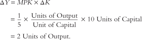
By increasing capital by 10 units, we obtain 2 more units of output. Thus, we use the marginal product of capital to convert changes in capital into changes in output.
Increases in Labour Next, consider changes in labour. If the amount of labour increases by ΔL units, by how much does output increase? We answer this question the same way we answered the question about capital. The marginal product of labour MPL tells us how much output changes when labour increases by 1 unit—that is,
MPL = F(K, L + 1) – F(K, L).
Therefore, when the amount of labour increases by ΔL units, output increases by approximately MPL × ΔL.
For example, suppose that the marginal product of labour is 2; that is, an additional unit of labour increases the amount of output produced by 2 units. If we increase the amount of labour by 10 units, we can compute the amount of additional output as follows:
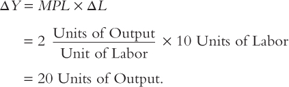
By increasing labour by 10 units, we obtain 20 more units of output. Thus, we use the marginal product of labour to convert changes in labour into changes in output.
Increases in Capital and Labour Finally, let’s consider the more realistic case in which both factors of production change. Suppose that the amount of capital increases by ΔK and the amount of labour increases by ΔL. The increase in output then comes from two sources: more capital and more labour. We can divide this increase into the two sources using the marginal products of the two inputs:
ΔY = (MPK × ΔK) + (MPL × ΔL).
The first term in parentheses is the increase in output resulting from the increase in capital, and the second term in parentheses is the increase in output resulting from the increase in labour. This equation shows us how to attribute growth to each factor of production.
282
We now want to convert this last equation into a form that is easier to interpret and apply to the available data. First, with some algebraic rearrangement, the equation becomes18
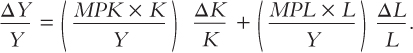
This form of the equation relates the growth rate of output, ΔY/Y, to the growth rate of capital, ΔK/K, and the growth rate of labour, ΔL/L.
Next, we need to find some way to measure the terms in parentheses in the last equation. In Chapter 3 we showed that the marginal product of capital equals its real rental price. Therefore, MPK × K is the total return to capital, and (MPK × K)/Y is capital’s share of output. Similarly, the marginal product of labour equals the real wage. Therefore, MPL × L is the total compensation that labour receives, and (MPL × L)/Y is labour’s share of output. Under the assumption that the production function has constant returns to scale, Euler’s theorem (which we discussed in Chapter 3) tells us that these two shares sum to 1. In this case, we can write
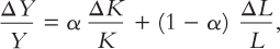
where α is capital’s share and (1 − α) is labour’s share.
This last equation gives us a simple formula for showing how changes in inputs lead to changes in output. In particular, we must weight the growth rates of the inputs by the factor shares. As we discussed in Chapter 3, capital’s share in Canada is about 33 percent, that is, α= 0.33. Therefore, a 10-percent increase in the amount of capital (DK/K = 0.10) leads to a 3.3-percent increase in the amount of output (ΔY/Y = 0.033). Similarly, a 10-percent increase in the amount of labour (ΔL/L = 0.10) leads to a 6.7-percent increase in the amount of output (ΔY/Y = 0.067).
Technological Progress
So far in our analysis of the sources of growth, we have been assuming that the production function does not change over time. In practice, of course, technological progress improves the production function. For any given amount of inputs, we can produce more output today than we could in the past. We now extend the analysis to allow for technological progress.
We include the effects of the changing technology by writing the production function as
Y = AF(K, L),
where A is a measure of the current level of technology called total factor productivity. Output now increases not only because of increases in capital and labour but also because of increases in total factor productivity. If total factor productivity increases by 1 percent and if the inputs are unchanged, then output increases by 1 percent.
283
Allowing for a changing technology adds another term to our equation accounting for economic growth:
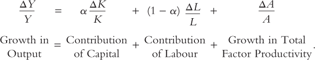
This is the key equation of growth accounting. It identifies and allows us to measure the three sources of growth: changes in the amount of capital, changes in the amount of labour, and changes in total factor productivity.
Because total factor productivity is not directly observable, it is measured indirectly. We have data on the growth in output, capital, and labour; we also have data on capital’s share of output. From these data and the growth-accounting equation, we can compute the growth in total factor productivity to make sure that everything adds up:
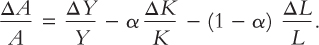
ΔA/A is the change in output that cannot be explained by changes in inputs. Thus, the growth in total factor productivity is computed as a residual—that is, as the amount of output growth that remains after we have accounted for the determinants of growth that we can measure. Indeed, ΔA/A is sometimes called the Solow residual, after Robert Solow, who first showed how to compute it.19
Total factor productivity can change for many reasons. Changes most often arise because of increased knowledge about production methods, so the Solow residual is often used as a measure of technological progress. Yet other factors, such as education and government regulation, can affect total factor productivity as well. For example, if higher public spending raises the quality of education, then workers may become more productive and output may rise, which implies higher total factor productivity. As another example, if government regulations require firms to purchase capital to reduce pollution or increase worker safety, then the capital stock may rise without any increase in measured output, which implies lower total factor productivity. Total factor productivity captures anything that changes the relation between measured inputs and measured output.
The Sources of Growth in Canada
Having learned how to measure the sources of economic growth, we now consider the data. On average, over the course of the twentieth century, Canadian output has grown at an annual rate of approximately 3 percent. Roughly speaking, over the same period, labour and capital have grown annually at 1 percentage point and 3 percentage points, respectively. Taking α at 0.33, we can provide rough estimates of the contribution to output growth of its three main determinants—growth in the labour input, growth in the capital input, and technological change. (The contribution of the latter is calculated as the residual). Table 8-3 shows the results.
284
We see that about 44 percent of the increase in Canadian output has been due to increases in productivity. More detailed estimates of this breakdown and evidence for subperiods within the century are available.20 These studies show that the contribution of increased productivity to growth has been as low as 23 percent and as high as 69 percent (in particular periods), but the average is the 44 percent that we have calculated above. It is in the last quarter of the twentieth century that the contribution of productivity growth was the smallest. This means that Canada’s slower average growth rate during this period had more to do with slower productivity growth than it did with a drop in the level of investment in new capital equipment. This fact makes it difficult to argue that all Canada needs to return to more rapid growth is to increase the rate of saving and investment spending.
As already noted, since the early 1970s, Canada’s overall productivity performance has lagged behind that of our competitors, in particular, that of the United States. The importance of lagging productivity growth for the competitiveness of Canadian firms can be appreciated by considering the final decade of the twentieth century. Over this decade, the wages of Canadian workers increased by 3 percent more than the wages of American workers. Canadian firms are less competitive if their unit labour costs rise compared to their competitors. If our workers had become more productive, the higher wages would not have increased unit costs. However, over the decade, productivity grew by 8 percent more in the United States, so—ignoring changes in the exchange rate—Canadian unit costs rose by 11 percent. Our firms remained competitive, however, since the Canadian dollar depreciated by almost double this amount during the 1990s. There has been increased concern about the gap between U.S. and Canadian productivity growth in recent years as the Canadian dollar has appreciated. In that environment, we no longer had the exchange rate acting as a cushion for our weaker productivity growth performance. As this book goes to press, however, the Canadian dollar is depreciating again, so our export firms are reacquiring some competitiveness.
| Source of Growth | Components | Data | Share of Output Growth |
| Output growth | ΔY/Y | 3% | |
| Labour’s share | (1 – α) times | 0.67 | |
| Labour growth rate | ΔL/L | 1% | |
| Contribution of labour | 0.67 | ||
| Capital’s share | α times | 0.33 | |
| Capital growth rate | ΔK/K | 3% | |
| Contribution of capital | 0.99 | ||
| Contribution of productivity growth | ΔY/Y – (1 – α)(ΔL/L) – α(ΔK/K) | 1.34 | |
| Proportion of growth due to increase in total factor productivity = 1.34/3 = 0.44 | |||
|
Source: Authors’ calculations. |
|||
|---|---|---|---|
285
CASE STUDY
Growth in the East Asian Tigers
Perhaps the most spectacular growth experiences in recent history have been those of the “Tigers” of East Asia: Hong Kong, Singapore, South Korea, and Taiwan. From 1966 to 1990, while real income per person was growing about 2 percent per year in the United States, it grew more than 7 percent per year in each of these countries. In the course of a single generation, real income per person increased fivefold, moving the Tigers from among the world’s poorest countries to among the richest. (In the late 1990s, a period of pronounced financial turmoil tarnished the reputation of some of these economies. But this short-run problem, which we examine in a case study in Chapter 12, doesn’t come close to reversing the spectacular long-run growth performance that the Asian Tigers have experienced.)
What accounts for these growth miracles? Some commentators have argued that the success of these four countries is hard to reconcile with basic growth theory, such as the Solow growth model, which takes technology as growing at a constant, exogenous rate. They have suggested that these countries’ rapid growth is due to their ability to imitate foreign technologies. By adopting technology developed abroad, the argument goes, these countries managed to improve their production functions substantially in a relatively short period of time. If this argument is correct, these countries should have experienced unusually rapid growth in total factor productivity.
One recent study shed light on this issue by examining in detail the data from these four countries. The study found that their exceptional growth can be traced to large increases in measured factor inputs: increases in labour-force participation, increases in the capital stock, and increases in educational attainment. In South Korea, for example, the investment–GDP ratio rose from about 5 percent in the 1950s to about 30 percent in the 1980s; the percentage of the working population with at least a high-school education went from 26 percent in 1966 to 75 percent in 1991.
Once we account for growth in labour, capital, and human capital, little of the growth in output is left to explain. None of these four countries experienced unusually rapid growth in total factor productivity. Indeed, the average growth in total factor productivity in the East Asian Tigers was almost exactly the same as in the United States. Thus, although these countries’ rapid growth has been truly impressive, it is easy to explain using the tools of basic growth theory.21 
The Solow Residual in the Short Run
286
When Robert Solow introduced his famous residual, his aim was to shed light on the forces that determine technological progress and economic growth in the long run. But economist Edward Prescott has used American data to look at the Solow residual as a measure of technological change over shorter periods of time. He concludes that fluctuations in technology are a major source of short-run changes in economic activity.
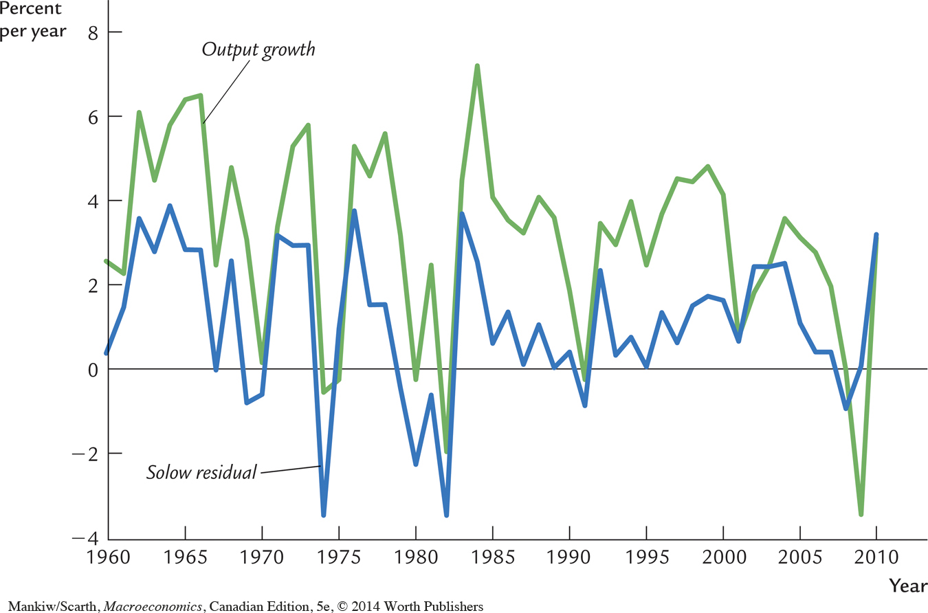
Figure 8-2 shows the Solow residual and the growth in output using annual data for the United States during the period 1960 to 2010. Notice that the Solow residual fluctuates substantially. If Prescott’s interpretation is correct, then we can draw conclusions from these short-run fluctuations, such as that technology worsened in 1982 and improved in 1984. Notice also that the Solow residual moves closely with output: in years when output falls, technology tends to worsen. In Prescott’s view, this fact implies that recessions are driven by adverse shocks to technology. The hypothesis that technological shocks are the driving force behind short-run economic fluctuations, and the complementary hypothesis that monetary policy has no role in explaining these fluctuations, form the foundation for an approach called real-business-cycle theory.
Prescott’s interpretation of these data is controversial, however. Many economists believe that the Solow residual does not accurately represent changes in technology over short periods of time. The standard explanation of the cyclical behaviour of the Solow residual is that it results from two measurement problems.
First, during recessions, firms may continue to employ workers they do not need so that they will have these workers on hand when the economy recovers. This phenomenon, called labour hoarding, means that labour input is overestimated in recessions, because the hoarded workers are probably not working as effectively as usual. As a result, the Solow residual is more cyclical than the available production technology. In a recession, productivity as measured by the Solow residual falls even if technology has not changed simply because hoarded workers are sitting around waiting for the recession to end.
Second, when demand is low, firms may produce things that are not easily measured. In recessions, workers may clean the factory, organize the inventory, get some training, and do other useful tasks that standard measures of output fail to include. If so, then output is underestimated in recessions, which would also make the measured Solow residual cyclical for reasons other than technology.
287
Thus, economists can interpret the cyclical behavior of the Solow residual in different ways. Some economists point to the low productivity in recessions as evidence for adverse technology shocks. Others believe that measured productivity is low in recessions because workers are not working as hard as usual and because more of their output is not measured. Unfortunately, there is no clear evidence on the importance of labour hoarding and the cyclical mismeasurement of output. Therefore, different interpretations of Figure 8-2 persist.22