291
Introduction to Economic Fluctuations
The modern world regards business cycles much as the ancient Egyptians regarded the overflowing of the Nile. The phenomenon recurs at intervals, it is of great importance to everyone, and natural causes of it are not in sight.
— John Bates Clark, 1898
Economic fluctuations present a recurring problem for economists and policymakers. On average, Canada’s real GDP has grown at an annual rate of 3.1 percent since 1970, but this long-run average hides the fact that the economy’s output of goods and services has not grown smoothly. Growth is higher in some years than in others; sometimes the economy loses ground and growth turns negative. These fluctuations in the economy’s output are closely associated with fluctuations in employment. When the economy experiences a period of falling output and rising unemployment, the economy is said to be in recession. Recessions occurred in 1991 and 2009. As you can see in Figure 9-1, real GDP fell about 2 percent in the first of these recessions, and then by almost 4 percent in the second. Not surprisingly, the unemployment rate rose over this period, from 7.5 percent in 1989 to 11.3 percent in 1992, and by about 2.5 percentage points in the recent recession. Often one of the most important drivers of fluctuations in the Canadian economy is the existence of volatility in the United States. Because we export a significant fraction of our output to the Americans, when they stop buying Canadian goods, many firms in Canada need to cut production. But our economy is not a mirror image of the U.S. economy. For example, the recent recession has been deeper there. As a result, unemployment rose more dramatically south of the border. In addition to rising unemployment, recessions are also associated with shorter workweeks: more workers have part-time jobs, and fewer workers work overtime.
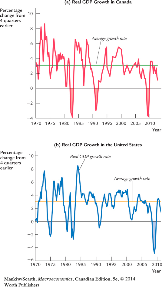
Economists call these fluctuations in output and employment the business cycle. Although this term suggests that fluctuations in the economy are regular and predictable, neither is the case, as Figure 9-1 makes clear. The historical fluctuations summarized in the figure raise a variety of related questions. What causes short-run fluctuations? What model should we use to explain them? Can policymakers avoid recessions? If so, what policy levers should they use?
292
293
In Parts Two and Three of this book, we developed models to identify the long-run determinants of national income, unemployment, inflation, and other economic variables. Yet we did not examine why these variables fluctuate so much from year to year. Here in Part Four, we see how economists explain short-run fluctuations. We begin in this chapter with two tasks. First, we discuss the key differences between how the economy behaves in the long run and how it behaves in the short run. Second, we introduce the model of aggregate supply and aggregate demand, which most economists use to explain short-run fluctuations. Developing this model in more detail will be our primary job in the chapters that follow.
Because real GDP is the best single measure of economic activity, it is the focus of our model. Yet you will recall from our discussion of Okun’s law near the end of Chapter 2, the business cycle is apparent not only in data from the national income accounts but also in data that describe conditions in the labour market. Put simply, when the economy heads into an economic downturn, jobs are harder to find. In Chapter 2 we saw that a temporary slowing of the GDP growth rate by 2 percentage points typically results in a 1 percentage point temporary rise in the unemployment rate. This is one of the primary reasons why policymakers are concerned about business cycles.
Okun’s law is a reminder that the forces governing the short-run business cycle are very different from those shaping long-run economic growth. As we saw in Chapters 7 and 8, long-run growth in GDP is determined primarily by technological progress. The long-run trend leading to higher standards of living from generation to generation is not associated with any long-run trend in the rate of unemployment. By contrast, short-run movements in GDP are highly correlated with the utilization of the economy’s labour force. The declines in the production of goods and services that occur during recessions are always associated with increases in joblessness.
Many economists, particularly those working in business and government, are engaged in the task of forecasting short-run fluctuations in the economy. Business economists are interested in forecasting to help their companies plan for changes in the economic environment. Government economists are interested in forecasting for two reasons. First, the economic environment affects the government; for example, the state of the economy influences how much tax revenue the government collects. Second, the government can affect the economy through its choice of monetary and fiscal policy. Economic forecasts are therefore an input into policy planning.
One way that economists arrive at their forecasts is by looking at leading indicators, which are variables that tend to fluctuate in advance of the overall economy. Forecasts can differ in part because economists hold varying opinions about which leading indicators are the most reliable. Some of the most used leading indicators are new orders, inventory levels, the number of new building permits issued, stock market indexes, money supply data, the spread between short-term and long-term interest rates, and consumer confidence surveys. These data are often used to forecast changes in economic activity about six to nine months into the future.
Other than looking at leading indicators, what can policymakers use to guide their deliberations? They can rely on the model of aggregate supply and demand that has been developed by macroeconomists. We now turn to the task of developing this framework.
Just as Egypt now controls the flooding of the Nile Valley with the Aswan Dam, modern society tries to control the business cycle with appropriate economic policies. The model we develop over the next several chapters shows how monetary and fiscal policies influence the business cycle. We will see that these policies can potentially stabilize the economy or, if poorly conducted, make the problem of economic instability even worse.