Aggregate demand (AD) is the relationship between the quantity of output demanded and the aggregate price level. In other words, the aggregate demand curve tells us the quantity of goods and services people want to buy at any given level of prices. We examine the theory of aggregate demand in detail in Chapters 10 through 12. Here we use the quantity theory of money to provide a simple, although incomplete, derivation of the aggregate demand curve.

Recall from Chapter 4 that the quantity theory says that

MV = PY,

where M is the money supply, V is the velocity of money, P is the price level, and Y is the amount of output. If the velocity of money is constant, then this equation states that the money supply determines the nominal value of output, which in turn is the product of the price level and the amount of output.

You might recall that the quantity equation can be rewritten in terms of the supply and demand for real money balances:

M/P = (M/P)^d = kY,

where k = 1/V is a parameter determining how much money people want to hold for every dollar of income. In this form, the quantity equation states that the supply of real money balances M/P equals the demand (M/P)^d and that the demand is proportional to output Y. The velocity of money V is the “flip side” of the money demand parameter k.

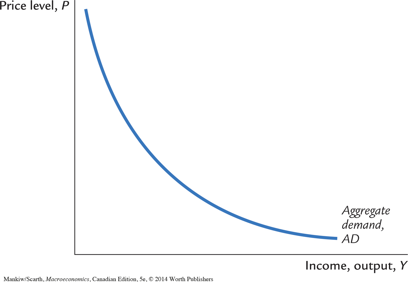
For any fixed money supply and velocity, the quantity equation yields a negative relationship between the price level P and output Y. Figure 9-2 graphs the combinations of P and Y that satisfy the quantity equation holding M and V constant. This downward-sloping curve is called the aggregate demand curve.

299

As a strictly mathematical matter, the quantity equation explains the downward slope of the aggregate demand curve very simply. The money supply M and the velocity of money V determine the nominal value of output PY. Once PY is fixed, if P goes up, Y must go down.

What is the economic intuition that lies behind this mathematical relationship? For a complete answer, we have to wait a couple of chapters. For now, however, consider the following logic: Because we have assumed that the velocity of money is fixed, the money supply determines the dollar value of all transactions in the economy. (This conclusion should be familiar from Chapter 4.) If the price level rises for some reason, so that each transaction requires more dollars, the number of transactions and thus the quantity of goods and services purchased must fall.

We can also explain the downward slope of the aggregate demand curve by thinking about the supply and demand for real money balances. If output is higher, people engage in more transactions and need higher real balances M/P. For a fixed money supply M, higher real balances imply a lower price level. Conversely, if the price level is lower, real money balances are higher; the higher level of real balances allows a greater volume of transactions, which means a greater quantity of output is demanded.

300

The aggregate demand curve is drawn for a fixed value of the money supply. In other words, it tells us the possible combinations of P and Y for a given value of M. If the money supply changes, then the possible combinations of P and Y change, which means the aggregate demand curve shifts.

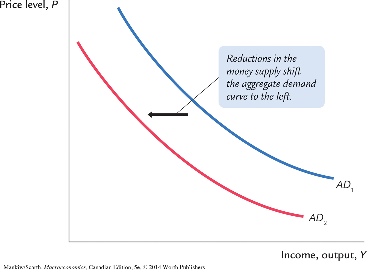
For example, consider what happens if the Bank of Canada reduces the money supply. The quantity equation, MV = PY, tells us that the reduction in the money supply leads to a proportionate reduction in the nominal value of output PY. For any given price level, the amount of output is lower, and for any given amount of output, the price level is lower. As in Figure 9-3, the aggregate demand curve relating P and Y shifts inward.

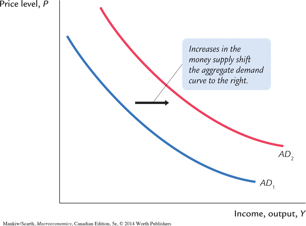
The opposite occurs if the Bank of Canada increases the money supply. The quantity equation tells us that an increase in M leads to an increase in PY. For any given price level, the amount of output is higher, and for any given amount of output, the price level is higher. As shown in Figure 9-4, the aggregate demand curve shifts outward.

Although the quantity theory of money gives a very simple basis for understanding the aggregate demand curve, be forewarned that reality is more complicated. Fluctuations in the money supply are not the only source of fluctuations in aggregate demand. Even if the money supply is held constant, the aggregate demand curve shifts if some event causes a change in the velocity of money. Over the next three chapters, we consider many possible reasons for shifts in the aggregate demand curve.