315
Aggregate Demand I: Building the IS–LM Model
I shall argue that the postulates of the classical theory are applicable to a special case only and not to the general case. . . . Moreover, the characteristics of the special case assumed by the classical theory happen not to be those of the economic society in which we actually live, with the result that its teaching is misleading and disastrous if we attempt to apply it to the facts of experience.
— John Maynard Keynes, The General Theory
Of all the economic fluctuations in world history, the one that stands out as particularly large, painful, and intellectually significant is the Great Depression of the 1930s. During this time, Canada and many other countries experienced massive unemployment and greatly reduced incomes. In the worst year, 1933, over one-fifth of the Canadian labour force was unemployed, and real GDP was 28 percent below its 1929 level.
This devastating episode caused many economists to question the validity of classical economic theory—the theory we examined in Chapters 3 through 8. Classical theory seemed incapable of explaining the Depression. According to that theory, national income depends on factor supplies and the available technology, neither of which changed substantially from 1929 to 1933. After the onset of the Depression, many economists believed that a new model was needed to explain such a large and sudden economic downturn and to suggest government policies that might reduce the economic hardship so many people faced.
In 1936 the British economist John Maynard Keynes revolutionized economics with his book The General Theory of Employment, Interest, and Money. Keynes proposed a new way to analyze the economy, which he presented as an alternative to classical theory. His vision of how the economy works quickly became a center of controversy. Yet, as economists debated The General Theory, a new understanding of economic fluctuations gradually developed.
Keynes proposed that low aggregate demand is responsible for the low income and high unemployment that characterize economic downturns. He criticized classical theory for assuming that aggregate supply alone—capital, labour, and technology—determines national income. Economists today reconcile these two views with the model of aggregate demand and aggregate supply introduced in Chapter 9. In the long run, prices are flexible, and aggregate supply determines income. But in the short run, prices are sticky, so changes in aggregate demand influence income. In 2008 and 2009, as all market economies descended into a recession, the Keynesian theory of business cycles was often in the news. Policymakers around the world debated how best to increase aggregate demand and put their economies on the road to recovery.
316
In this chapter and the next, we continue our study of economic fluctuations by looking more closely at aggregate demand. Our goal is to identify the variables that shift the aggregate demand curve, causing fluctuations in national income. We also examine more fully the tools policymakers can use to influence aggregate demand. In Chapter 9 we derived the aggregate demand curve from the quantity theory of money, and we showed that monetary policy can shift the aggregate demand curve. In this chapter we see that the government can influence aggregate demand with both monetary and fiscal policy.
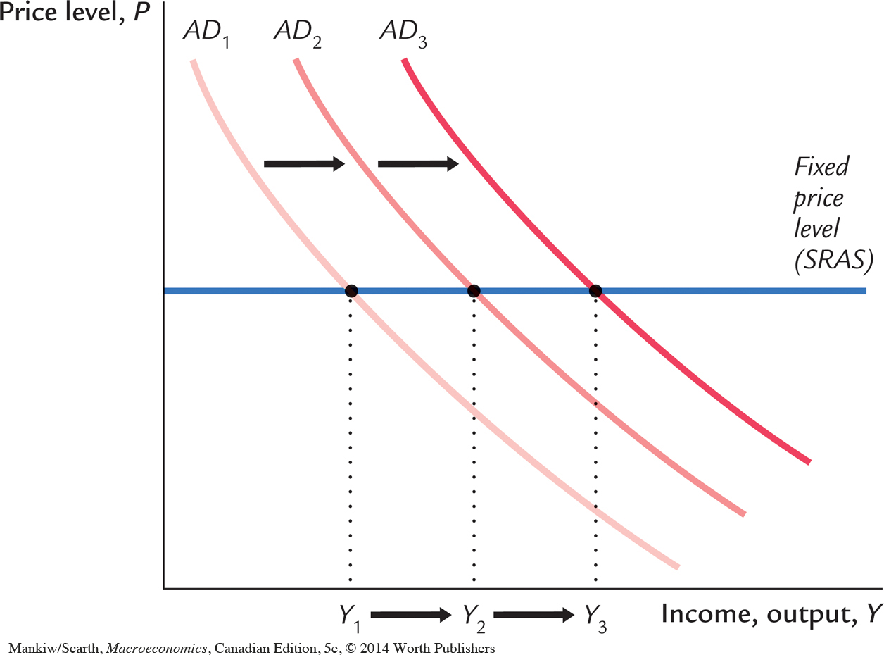
The model of aggregate demand developed in this chapter, called the IS–LM model, is the leading interpretation of Keynes’s theory. The goal of the model is to show what determines national income for any given price level. There are two ways to interpret this exercise. We can view the IS–LM model as showing what causes income to change in the short run when the price level is fixed. Or we can view the model as showing what causes the aggregate demand curve to shift. These two interpretations of the model are equivalent: as Figure 10-1 shows, in the short run when the price level is fixed, shifts in the aggregate demand curve lead to changes in national income.
The two parts of the IS–LM model are, not surprisingly, the IS curve and the LM curve. IS stands for “investment” and “saving,” and the IS curve represents what’s going on in the market for goods and services (which we first discussed in Chapter 3). LM stands for “liquidity” and “money,” and the LM curve represents what’s happening to the supply and demand for money (which we first discussed in Chapter 4). Because the interest rate influences both investment and money demand, it is the variable that links the two halves of the IS–LM model. The model shows how interactions between these markets determine the position and slope of the aggregate demand curve and, therefore, the level of national income in the short run.1