10.1 The Goods Market and the IS Curve
317
The IS curve plots the relationship between the interest rate and the level of income that arises in the market for goods and services. To develop this relationship, we start with a basic model called the Keynesian cross. This model is the simplest interpretation of Keynes’s theory of how national income is determined, and it is also a building block for the more complex and realistic IS–LM model.
The Keynesian Cross
In The General Theory Keynes proposed that an economy’s total income was, in the short run, determined largely by the desire to spend by households, firms, and the government. The more people want to spend, the more goods and services firms can sell. The more firms can sell, the more output they will choose to produce and the more workers they will choose to hire. Thus, the problem during recessions and depressions, according to Keynes, was inadequate spending. The Keynesian cross is an attempt to model this insight.
Planned Expenditure We begin our derivation of the Keynesian cross by drawing a distinction between actual and planned expenditure. Actual expenditure is the amount households, firms, and the government spend on goods and services, and as we first saw in Chapter 2, it equals the economy’s gross domestic product (GDP). Planned expenditure is the amount households, firms, and the government would like to spend on goods and services.
Why would actual expenditure ever differ from planned expenditure? The answer is that firms might engage in unplanned inventory investment because their sales do not meet their expectations. When firms sell less of their product than they planned, their stock of inventories automatically rises; conversely, when firms sell more than planned, their stock of inventories falls. Because these unplanned changes in inventory are counted as investment spending by firms, actual expenditure can be either above or below planned expenditure.
Now consider the determinants of planned expenditure. In this chapter, we simplify by assuming that the economy is closed, so that net exports are zero. Of course, Canada is an open economy that exports a significant portion of our GDP. Thus, while our simplifying assumption is very helpful in getting the discussion of aggregate demand theory started, we must extend it to the open-economy case later on. We devote an entire chapter (Chapter 12) to doing just that. In the meantime, we write planned expenditure PE as the sum of consumption C, planned investment I, and government purchases G:
318
PE = C + I + G.
To this equation, we add the consumption function
C = C(Y – T).
This equation states that consumption depends on disposable income (Y – T), which is total income Y minus taxes T. To keep things simple, for now we take planned investment as exogenously fixed:

And as in Chapter 3, we assume that fiscal policy—the levels of government purchases and taxes—is fixed:

Combining these five equations, we obtain

This equation shows that planned expenditure is a function of income Y, the level of planned investment  , and the fiscal policy variables
  and
and  .
.
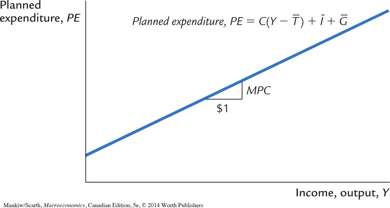
Figure 10-2 graphs planned expenditure as a function of the level of income. This line slopes upward because higher income leads to higher consumption and thus higher planned expenditure. The slope of this line is the marginal propensity to consume, the MPC: it shows how much planned expenditure increases when income rises by $1. This planned-expenditure function is the first piece of the model called the Keynesian cross.
319
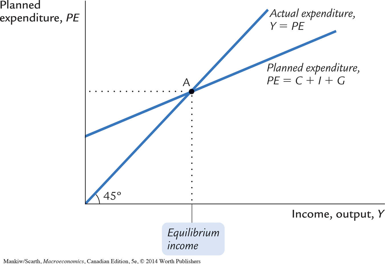
The Economy in Equilibrium The next piece of the Keynesian cross is the assumption that the economy is in equilibrium when actual expenditure equals planned expenditure. This assumption is based on the idea that when people’s plans have been realized, they have no reason to change what they are doing. Recalling that Y as GDP equals not only total income but also total actual expenditure on goods and services, we can write this equilibrium condition as
Actual Expenditure = Planned Expenditure
Y = PE.
The 45-degree line in Figure 10-3 plots the points where this condition holds. With the addition of the planned-expenditure function, this diagram becomes the Keynesian cross. The equilibrium of this economy is at point A, where the planned-expenditure function crosses the 45-degree line.
How does the economy get to the equilibrium? In this model, inventories play an important role in the adjustment process. Whenever the economy is not in equilibrium, firms experience unplanned changes in inventories, and this induces them to change production levels. Changes in production in turn influence total income and expenditure, moving the economy toward equilibrium.
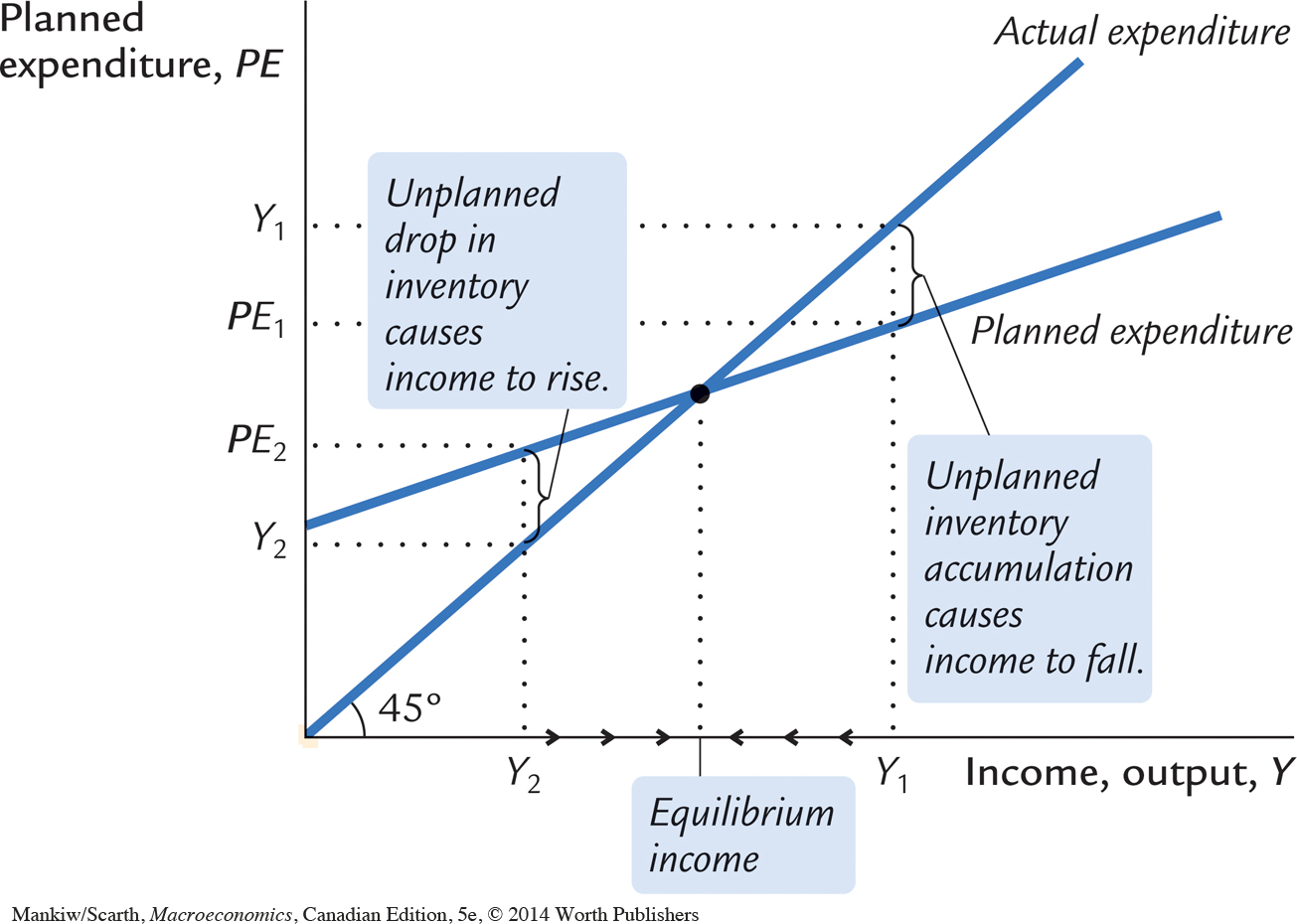
For example, suppose the economy were ever to find itself with GDP at a level greater than the equilibrium level, such as the level Y1 in Figure 10-4. In this case, planned expenditure PE1 is less than production Y1, so firms are selling less than they are producing. Firms add the unsold goods to their stock of inventories. This unplanned rise in inventories induces firms to lay off workers and reduce production, and these actions in turn reduce GDP. This process of unintended inventory accumulation and falling income continues until income Y falls to the equilibrium level.
320
Similarly, suppose GDP were at a level lower than the equilibrium level, such as the level Y2 in Figure 10-4. In this case, planned expenditure PE2 is greater than production Y2. Firms meet the high level of sales by drawing down their inventories. But when firms see their stock of inventories dwindle, they hire more workers and increase production. GDP rises, and the economy approaches the equilibrium.
In summary, the Keynesian cross shows how income Y is determined for given levels of planned investment I and fiscal policy G and T. We can use this model to show how income changes when one of these exogenous variables changes.
Fiscal Policy and the Multiplier: Government Purchases Consider how changes in government purchases affect the economy. Because government purchases are one component of expenditure, higher government purchases result in higher planned expenditure for any given level of income. If government purchases rise by ΔG, then the planned-expenditure schedule shifts upward by ΔG, as in Figure 10-5. The equilibrium of the economy moves from point A to point B.
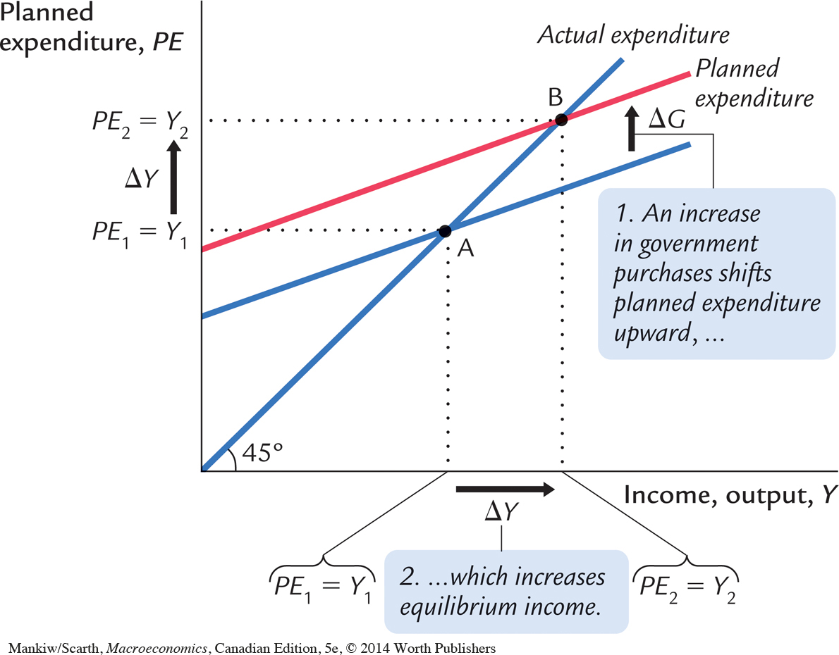

This graph shows that an increase in government purchases leads to an even greater increase in income. That is, ΔY is larger than ΔG. The ratio ΔY/ΔG is called the government-purchases multiplier; it tells us how much income rises in response to a $1 increase in government purchases. An implication of the Keynesian cross is that the government-purchases multiplier is larger than 1.
321
Why does fiscal policy have a multiplied effect on income? The reason is that, according to the consumption function, C = C(Y – T), higher income causes higher consumption. When an increase in government purchases raises income, it also raises consumption, which further raises income, which further raises consumption, and so on. Therefore, in this model, an increase in government purchases causes a greater increase in income.
How big is the multiplier? To answer this question, we trace through each step of the change in income. The process begins when expenditure rises by ΔG, which implies that income rises by ΔG as well. This increase in income in turn raises consumption by MPC × ΔG, where MPC is the marginal propensity to consume. This increase in consumption raises expenditure and income once again. This second increase in income of MPC × ΔG again raises consumption, this time by MPC × (MPC × ΔG), which again raises expenditure and income, and so on. This feedback from consumption to income to consumption continues indefinitely. The total effect on income is
| Initial Change in Government Purchases | = ΔG |
| First Change in Consumption | = MPC × ΔG |
| Second Change in Consumption | = MPC2 × ΔG |
| Third Change in Consumption | = MPC3 × ΔG |
| . | . |
| . | . |
| . | . |
| ΔY = (1 + MPC + MPC2 + MPC3 + . . .) ΔG. | |
322
The government-purchases multiplier is
ΔY/ΔG = 1 + MPC + MPC2 + MPC3 + . . .
This expression for the multiplier is an example of an infinite geometric series. A result from algebra allows us to write the multiplier as2
ΔY/ΔG = 1/(1 – MPC).
For example, if the marginal propensity to consume is 0.6, the multiplier is
ΔY/ΔG = 1 + 0.6 + 0.62 + 0.63 + . . .
= 1/(1 – 0.6)
= 2.5.
In this case, a $1.00 increase in government purchases raises equilibrium income by $2.50.3
Fiscal Policy and the Multiplier: Taxes Consider now how changes in taxes affect equilibrium income. A decrease in taxes of ΔT immediately raises disposable income Y – T by ΔT and, therefore, increases consumption by MPC × ΔT. For any given level of income Y, planned expenditure is now higher. As Figure 10-6 shows, the planned-expenditure schedule shifts upward by MPC × ΔT. The equilibrium of the economy moves from point A to point B.
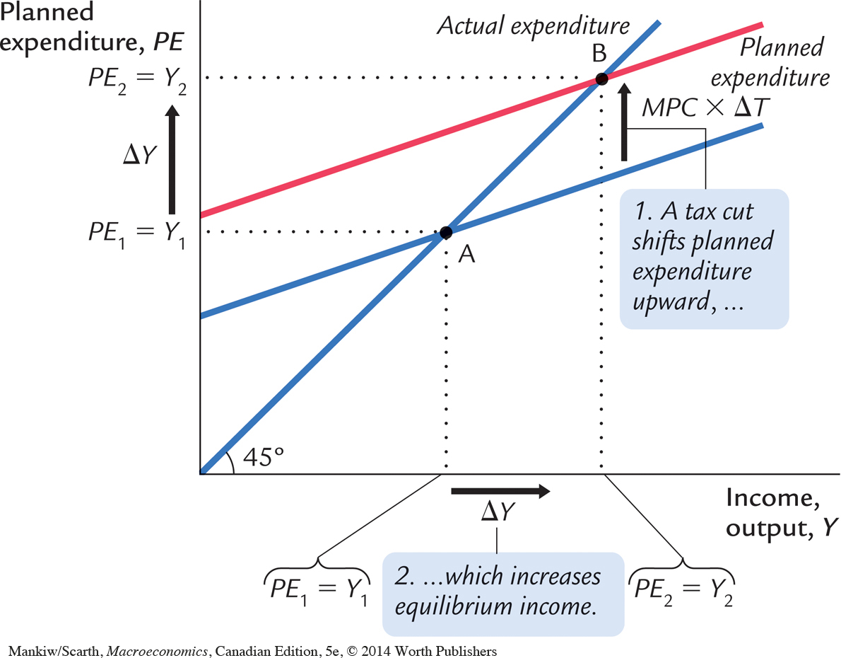
323
Just as an increase in government purchases has a multiplied effect on income, so does a decrease in taxes. As before, the initial change in expenditure, now MPC × ΔT, is multiplied by 1/(1 – MPC). The overall effect on income of the change in taxes is
ΔY/ΔT = –MPC/(1 – MPC).
This expression is the tax multiplier, the amount income changes in response to a $1 change in taxes. For example, if the marginal propensity to consume is 0.6, then the tax multiplier is
ΔY/ΔT = –0.6/(1 – 0.6) = –1.5.
In this example, a $1.00 cut in taxes raises equilibrium income by $1.50.4
324
CASE STUDY
Modest Expectations Concerning Job Creation
The Liberal Party formed Canada’s Government from 1993 to 2006. During the 1993 election, the Liberals campaigned on a platform of “jobs, jobs, jobs.” Many students, when hearing the term “multiplier,” expect that it could be fairly straightforward for governments to fulfull job-creation promises of this sort. But economists now believe that the multiplier terminology may create unrealistic expectations. This trend in thinking will become clearer as our understanding of aggregate demand progresses through this book. For example, we will be considering developments in financial markets—the effects of fiscal policy on interest rates and the exchange rate. We will learn that the size of our fiscal policy multipliers is much reduced by these considerations.
What is a plausible value for the government spending multiplier—given that, at this point, we must limit our attention to the simple formula 1/1 – MPC)? To answer this question, we must think of taxes, imports, and saving—the main things that keep a new dollar of income earned from being spent on domestically produced goods. The first consideration is the tax system; taxes increase by about $0.25 for each $1 increase in GDP. The second consideration is that the transfer payments people receive from the government decrease as their income increases, and in aggregate this variation means that transfer payments fall by about $0.15 for each $1 increase in GDP. Since “taxes” in our model stand for net payments by individuals to government—taxes less transfer receipts—we must take the overall “tax rate” to be 0.25 plus 0.15, or 0.40. Thus the proportion of income not taxed is 0.60. Finally, Canadians tend to import about one-quarter of all goods consumed. With a propensity to spend about 75 percent of each extra dollar of disposable income, we have an overall marginal propensity to consume domestically produced goods (out of each dollar of pretax income, GDP) equal to:
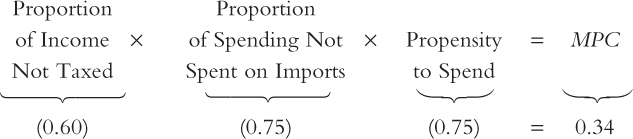
With the MPC estimated at 0.34, the spending multiplier, 1/1 – MPC), is 1.5.
The federal government’s deficit elimination program in the 1990s was the largest fiscal initiative undertaken in Canadian history—until that record was broken in 2009. During the 1994–1999 period, federal budgets involved an average cut in government spending of about $8 billion per year compared to what spending would have been if it had remained a constant fraction of GDP. Thus, we can take ΔG = $8 billion as representing the magnitude of the government’s fiscal policy during this period. The multiplier formula then predicts that ΔY is $12 billion. Since Canada’s GDP averaged $835 billion during these years, this fiscal policy involved changing output by about 1.4 percent.
325
How much could this initiative be expected to change unemployment? The answer to this question can be had by relying on Okun’s law, which was explained in Chapter 2. Okun’s law states that unemployment usually rises by about one-half the percentage fall in GDP. Thus, the effect of the fiscal policy of the 1990s is estimated to be a change in the unemployment rate of three-quarters of 1 percentage point. While that represented a little more than 100,000 jobs, with an average unemployment rate over this period of 9 percent, not many would summarize this change as “jobs, jobs, jobs.” We must also keep in mind that the simple formula, 1/(1 – MPC), overestimates the effects of policy.
It is also important to realize that a small multiplier was exactly what the government wanted during this period. Since the government was cutting expendentures to reduce the budget deficit, it did not want to destroy many jobs. A small fiscal multiplier was just what was needed in that case.
So the “jobs, jobs, jobs” electoral refrain was misleading for two reasons. First, because our fiscal policy multiplier is small, we must have modest expectations when governments use expansionary fiscal policy. Second, since the Liberals conducted a contractionary—not an expansionary—fiscal policy after being elected, jobs were destroyed, not created! 
CASE STUDY
The 2009 Stimulus Package
A world-wide recession developed in late 2008 (and we discuss the causes of this recession in a case study in the next chapter). In the face of this slow-down in economic activity, our federal government reversed its earlier promise to avoid running any budget deficit; in fact, its budget of January 2009 included a major fiscal stimulus. Along with the funds that provincial governments would spend as part of the programs, the government promised just over $50 billion of new program spending and tax cuts over the next two years—a total representing 3.5 percent of GDP. Roughly three-quarters of the initiatives involved increased government spending, and the remaining quarter was made up of tax cuts. An even larger fiscal initiative amounting to 5 percent of GDP was introduced at the same time in the United States, where President Obama’s full commitment to Keynesian analysis held sway.
We can use our analysis to assess whether the size of our government’s initiative was appropriate. Recalling from the previous case study that the fiscal-policy multiplier is certainly no larger than 1.5, we can appreciate that, while leading to a record budget deficit, our government’s stimulus was barely big enough to cope with the magnitude of the recession. Assuming that the $50 billion would be dispersed evenly over the two years, and ignoring the fact that the tax-multiplier is smaller than the spending multiplier, each annual initiative of $25 billion could be expected to raise GDP by (1.5 times $25 billion) = $37.5 billion—roughly 2.6 percent of GDP. During the final quarter of 2008 and the first quarter of 2009, Canadian GDP shrank by 3 percent, measured at annual rates. Thus, if policymakers were expecting at least two more quarters of recession, the policy in the budget could be assessed as barely adequate.
326
Much debate centred on whether the government should have stressed spending increases so much more than tax cuts. Advocates of the government’s decision argued that increased spending was better than reduced taxes because, according to standard Keynesian theory, the government-purchases multiplier exceeds the tax multiplier. The reason for this difference is simple: when the government spends one dollar, that dollar gets spent, whereas when the government gives households a tax cut of one dollar, that dollar or some of it might be saved. Thus, advocates argued, increased government spending on roads, schools, and other infrastructure was the better route to increase aggregate demand and create jobs. Other economists were more skeptical. One concern was that spending on infrastructure would take time, whereas tax cuts could occur more quickly. Infrastructure spending requires taking bids and signing contracts, and even after the projects begin, they can take years to complete. Past estimates indicate that, on average, it takes 18 months for the spending to start! With such lags, by the time much of the stimulus goes into effect, the recession might be long over.
In addition, some economists thought that using infrastructure spending to promote employment might conflict with the goal of obtaining the infrastructure that was most needed. Here is how Gary Becker, a Nobel Prize-winning economist, explained the concern on his blog:
Putting new infrastructure spending in depressed areas like Detroit might have a big stimulating effect since infrastructure building projects in these areas can utilize some of the considerable unemployed resources there. However, many of these areas are also declining because they have been producing goods and services that are not in great demand, and will not be in demand in the future. Therefore, the overall value added by improving their roads and other infrastructure is likely to be a lot less than if the new infrastructure were located in growing areas that might have relatively little unemployment, but do have great demand for more roads, schools, and other types of long-term infrastructure.
In its budget, the government stressed the three desirable features of a fiscal initiative—that it be timely, targeted, and temporary. Finance Canada officials argued that spending initiatives could be targeted more easily on depressed sectors or regions than could general tax cuts. Admittedly, however, some tax cuts, such as the expansion of the Working Income Tax Benefit which was part of the 2009 budget, are easily targeted on the least well-off working Canadians. Nevertheless, while the infrastructure projects score well on the targeted criterion overall, they score lower on being timely, as we have already noted. Finally, there is the temporary criterion—a question of how easy or difficult it is to reverse an initiative. The whole point of a policy of aggregate-demand management is that it is temporary. We want a stimulus only during the recession phase of the business cycle, a limitation that is very difficult to maintain with tax cuts. Once a tax cut is enacted, it is politically very hard to end. It is much easier to end infrastructure spending simply by not starting an additional project once the previous one has been completed.
327
Although the government did not make a persuasive case that it had struck a perfect balance between the advantages and disadvantages of spending increases versus tax cuts—in terms of all three of the important timely, targeted and temporary criteria—we can at least appreciate the nature of the compromises it faced. But whatever the details, policy-makers clearly have accepted the economic intuition provided by our basic short-run model of aggregate demand. The logic that actual fiscal-policy practitioners use is quintessentially Keynesian: when the economy sinks into recession, most governments seem to embrace the notion to act as demanders of last resort, despite small fiscal-policy multipliers and challenges of timing and reversibility.
In future chapters we will return to the broad question of whether governments should conduct an active stabilization policy—after we identify several other challenges by extending the theory of aggregate supply and demand.
The Interest Rate, Investment, and the IS Curve
The Keynesian cross is only a steppingstone on our path to the IS–LM model. The Keynesian cross is useful because it shows how the spending plans of households, firms, and the government determine the economy’s income. Yet it makes the simplifying assumption that the level of planned investment I is fixed. As we discussed in Chapter 3, an important macroeconomic relationship is that planned investment depends on the interest rate r.
To add this relationship between the interest rate and investment to our model, we write the level of planned investment as
I = I(r).
This investment function is graphed in panel (a) of Figure 10-7. Because the interest rate is the cost of borrowing to finance investment projects, an increase in the interest rate reduces planned investment. As a result, the investment function slopes downward.
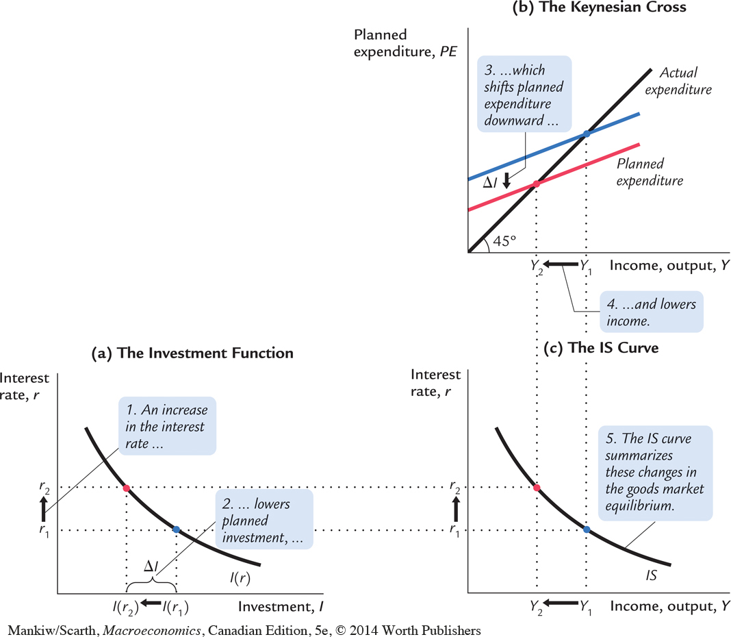
To determine how income changes when the interest rate changes, we can combine the investment function with the Keynesian-cross diagram. Because investment is inversely related to the interest rate, an increase in the interest rate from r1 to r2 reduces the quantity of investment from I(r1) to I(r2). The reduction in planned investment, in turn, shifts the planned-expenditure function downward, as in panel (b) of Figure 10-7. The shift in the planned-expenditure function causes the level of income to fall from Y1 to Y2. Hence, an increase in the interest rate lowers income.
The IS curve, shown in panel (c) of Figure 10-7, summarizes this relationship between the interest rate and the level of income. In essence, the IS curve combines the interaction between r and I expressed by the investment function and the interaction between I and Y demonstrated by the Keynesian cross. Because an increase in the interest rate causes planned investment to fall, which in turn causes income to fall, the IS curve slopes downward.
How Fiscal Policy Shifts the IS Curve
328
The IS curve shows us, for any given interest rate, the level of income that brings the goods market into equilibrium. As we learned from the Keynesian cross, the level of income also depends on fiscal policy. The IS curve is drawn for a given fiscal policy; that is, when we construct the IS curve, we hold G and T fixed. When fiscal policy changes, the IS curve shifts.
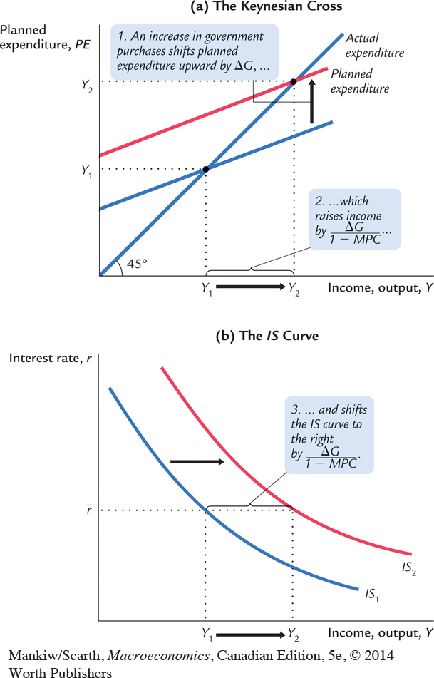
Figure 10-8 uses the Keynesian cross to show how an increase in government purchases from G1 to G2 shifts the IS curve. This figure is drawn for a given interest rate  and thus for a given level of planned investment. The Keynesian cross shows that this change in fiscal policy raises planned expenditure and thereby increases equilibrium income from Y1 to Y2. Therefore, an increase in government purchases shifts the IS curve outward.
We can use the Keynesian cross to see how other changes in fiscal policy shift the IS curve. Because a decrease in taxes also expands expenditure and income, it too shifts the IS curve outward. A decrease in government purchases or an increase in taxes reduces income; therefore, such a change in fiscal policy shifts the IS curve inward.
329
In summary, the IS curve shows the combinations of the interest rate and the level of income that are consistent with equilibrium in the market for goods and services. The IS curve is drawn for a given fiscal policy. Changes in fiscal policy that raise the demand for goods and services shift the IS curve to the right. Changes in fiscal policy that reduce the demand for goods and services shift the IS curve to the left.
A Loanable-Funds Interpretation of the IS Curve
330
When we first studied the market for goods and services in Chapter 3, we noted an equivalence between the supply and demand for goods and services and the supply and demand for loanable funds. This equivalence provides another way to interpret the IS curve.
Recall that the national accounts identity can be written as
Y – C – G = I
S = I.
The left-hand side of this equation is national saving S, and the right-hand side is investment I. National saving represents the supply of loanable funds, and investment represents the demand for these funds.
To see how the market for loanable funds produces the IS curve, substitute the consumption function for C and the investment function for I:
Y – C(Y – T) – G = I(r).
The left-hand side of this equation shows that the supply of loanable funds depends on income and fiscal policy. The right-hand side shows that the demand for loanable funds depends on the interest rate. The interest rate adjusts to equilibrate the supply and demand for loans.
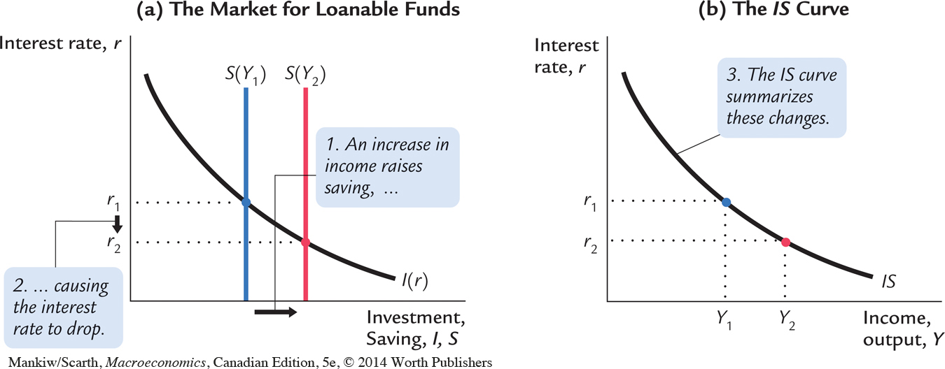
As Figure 10-9 illustrates, we can interpret the IS curve as showing the interest rate that equilibrates the market for loanable funds for any given level of income. When income rises from Y1 to Y2, national saving, which equals Y – C – G, increases. (Consumption rises by less than income, because the marginal propensity to consume is less than 1.) As panel (a) shows, the increased supply of loanable funds drives down the interest rate from r1 to r2. The IS curve in panel (b) summarizes this relationship: higher income implies higher saving, which in turn implies a lower equilibrium interest rate. For this reason, the IS curve slopes downward.
331
This alternative interpretation of the IS curve also explains why a change in fiscal policy shifts the IS curve. An increase in government purchases or a decrease in taxes reduces national saving for any given level of income. The reduced supply of loanable funds raises the interest rate that equilibrates the market. Because the interest rate is now higher for any given level of income, the IS curve shifts upward in response to the expansionary change in fiscal policy.
Finally, note that the IS curve does not determine either income Y or the interest rate r. Instead, the IS curve is a relationship between Y and r arising in the market for goods and services or, equivalently, the market for loanable funds. Recall that our goal in this chapter is to understand aggregate demand; that is, we want to find what determines equilibrium income Y for a given price level P. The IS curve is just half the story. To complete the story, we need another relationship between Y and r, to which we now turn.