10.2 The Money Market and the LM Curve
The LM curve plots the relationship between the interest rate and the level of income that arises in the market for money balances. To understand this relationship, we begin by looking at a theory of the interest rate, called the theory of liquidity preference.
The Theory of Liquidity Preference
In his classic work The General Theory, Keynes offered his view of how the interest rate is determined in the short run. His explanation is called the theory of liquidity preference, because it posits that the interest rate adjusts to balance the supply and demand for the economy’s most liquid asset—money. Just as the Keynesian cross is a building block for the IS curve, the theory of liquidity preference is a building block for the LM curve.
To develop this theory, we begin with the supply of real money balances. If M stands for the supply of money and P stands for the price level, then M/P is the supply of real money balances. The theory of liquidity preference assumes there is a fixed supply of real balances. That is,
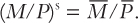
The money supply M is an exogenous policy variable chosen by a central bank, such as the Bank of Canada. The price level P is also an exogenous variable in this model. (We take the price level as given because the IS–LM model—our ultimate goal in this chapter—explains the short run when the price level is fixed.) These assumptions imply that the supply of real balances is fixed and, in particular, does not depend on the interest rate. Thus, when we plot the supply of real money balances against the interest rate in Figure 10-10, we obtain a vertical supply curve.
332
Next, consider the demand for real money balances. The theory of liquidity preference posits that the interest rate is one determinant of how much money people choose to hold. The underlying reason is that the interest rate is the opportunity cost of holding money: it is what you forgo by holding some of your assets as money, which does not bear interest, instead of as interest-bearing bank deposits or bonds. When the interest rate rises, people want to hold less of their wealth in the form of money. Thus, we can write the demand for real money balances as
(M/P)d = L(r),
where the function L(r) shows that the quantity of money demanded depends on the interest rate. The demand curve in Figure 10-10 illustrates this relationship. This demand curve slopes downward because higher interest rates reduce the quantity of real balances demanded.5
According to the theory of liquidity preference, the interest rate adjusts to equilibrate the money market. As Figure 10-10 shows, at the equilibrium interest rate, the quantity of real balances demanded equals the quantity supplied.
333
How does the interest rate get to this equilibrium of money supply and money demand? The adjustment occurs because whenever the money market is not in equilibrium, people try to adjust their portfolios of assets and, in the process, alter the interest rate. For instance, if the interest rate is above the equilibrium level, the quantity of real balances supplied exceeds the quantity demanded. Individuals holding the excess supply of money try to convert some of their non-interest-bearing money into interest-bearing bank deposits or bonds. Banks and bond issuers, who prefer to pay lower interest rates, respond to this excess supply of money by lowering the interest rates they offer. Conversely, if the interest rate is below the equilibrium level, so that the quantity of money demanded exceeds the quantity supplied, individuals try to obtain money by selling bonds or making bank withdrawals. To attract now scarcer funds, banks and bond issuers respond by increasing the interest rates they offer. Eventually, the interest rate reaches the equilibrium level, at which people are content with their portfolios of monetary and nonmonetary assets.
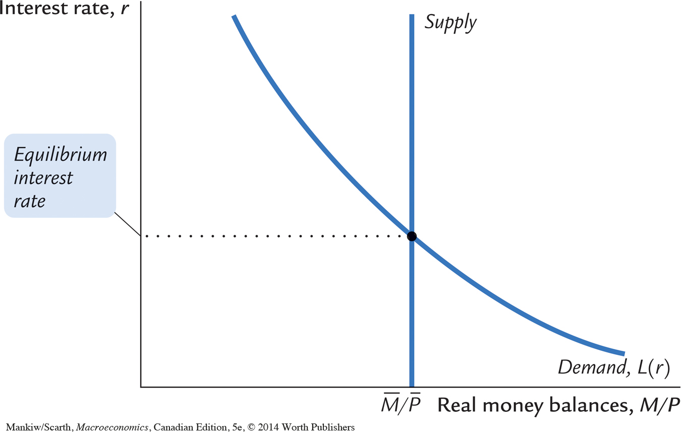
Now that we have seen how the interest rate is determined, we can use the theory of liquidity preference to show how the interest rate responds to changes in the supply of money. Suppose, for instance, that the Bank of Canada suddenly decreases the money supply. A fall in M reduces M/P, because P is fixed in the model. The supply of real balances shifts to the left, as in Figure 10-11. The equilibrium interest rate rises from r1 to r2, and the higher interest rate makes people satisfied to hold the smaller quantity of real money balances. The opposite would occur if the Bank of Canada had suddenly increased the money supply. Thus, according to the theory of liquidity preference, a decrease in the money supply raises the interest rate, and an increase in the money supply lowers the interest rate.
334
CASE STUDY
Tight Money and Rising Interest Rates
The early 1980s saw a large and speedy reduction in North American inflation rates. During the 1980–1982 period, Canada’s CPI increased at an average annual rate of 11.2 percent; during the next three years, that rate of increase slowed to 4.7 percent. This 6.5-percentage-point reduction in inflation was achieved by a dramatic tightening of monetary policy.
During the 1970s, the quantity of real money balances (M1 divided by the CPI) had been growing at an average rate of 2.8 percent per year. Then, during the 1980–1982 period, Canadian real money growth was pushed down to an average of –7.8 percent per year. After that, monetary policy was eased significantly; average growth in real balances was 1.7 percent per year in the 1983–1985 period.
How does such a monetary tightening influence interest rates? The answer depends on the time horizon. Our analysis of the Fisher effect in Chapter 4 suggests that the change in monetary policy would lower inflation in the long run, which, in turn, would lead to lower nominal interest rates. Yet the theory of liquidity preference that we have considered in the present chapter predicts that, in the short run when prices are sluggish, anti-inflationary monetary policy involves a leftward shift of the money supply curve and higher nominal interest rates.
Both conclusions are consistent with experience. Nominal interest rates did fall in the 1980s as inflation fell. For example, the three-month treasury bill rate fell from an average of 14.7 percent in the 1980–1982 period to an average of 10 percent in the 1983–1985 period. But it is instructive to consider the year-to-year sequence. The interest rate rose from 12.7 percent in 1980 to 17.8 percent in 1981, and it did not fall below 12.7 percent until 1983. The moral of the story is that both our short-run and our long-run analyses of interest-rate determination help us to understand the real world.
Income, Money Demand, and the LM Curve
Having developed the theory of liquidity preference as an explanation for how the interest rate is determined, we can now use the theory to derive the LM curve. We begin by considering the following question: how does a change in the economy’s level of income Y affect the market for real money balances? The answer (which should be familiar from Chapter 4) is that the level of income affects the demand for money. When income is high, expenditure is high, so people engage in more transactions that require the use of money. Thus, greater income implies greater money demand. We can express these ideas by writing the money demand function as
(M/P)d = L(r, Y).
The quantity of real money balances demanded is negatively related to the interest rate and positively related to income.
335
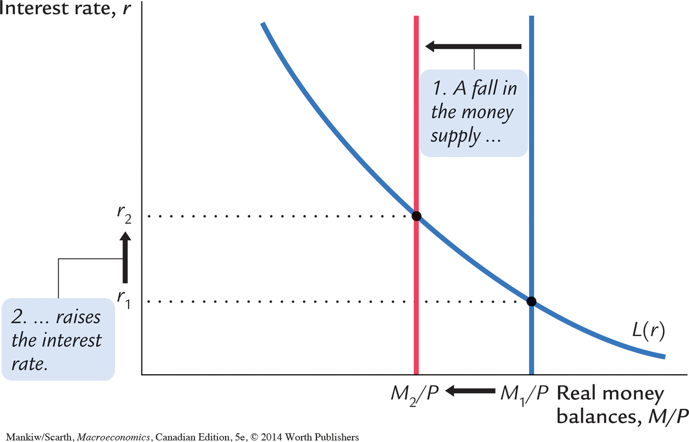
Using the theory of liquidity preference, we can figure out what happens to the equilibrium interest rate when the level of income changes. For example, consider what happens in Figure 10-12 when income increases from Y1 to Y2. As panel (a) illustrates, this increase in income shifts the money demand curve to the right. With the supply of real money balances unchanged, the interest rate must rise from r1 to r2 to equilibrate the money market. Therefore, according to the theory of liquidity preference, higher income leads to a higher interest rate.
The LM curve plots this relationship between the level of income and the interest rate. The higher the level of income, the higher the demand for real money balances, and the higher the equilibrium interest rate. For this reason, the LM curve slopes upward, as in panel (b) of Figure 10-12.
How Monetary Policy Shifts the LM Curve
The LM curve tells us the interest rate that equilibrates the money market at any level of income. Yet, as we saw earlier, the equilibrium interest rate also depends on the supply of real balances, M/P. This means that the LM curve is drawn for a given supply of real money balances. If real balances change—for example, if the Central Bank alters the money supply—the LM curve shifts.
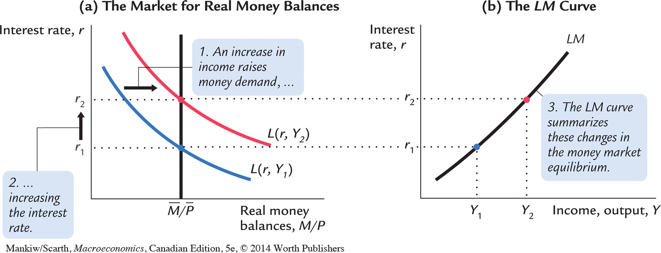
We can use the theory of liquidity preference to understand how monetary policy shifts the LM curve. Suppose that the Bank of Canada decreases the monetary base, which leads to a decrease in the money supply from M1 to M2. This development causes the supply of real balances to fall from M1/P to M2/P. Figure 10-13 shows what happens. Holding constant the amount of income and thus the demand curve for real balances, we see that a reduction in the supply of real balances raises the interest rate that equilibrates the money market. Hence, a decrease in real balances shifts the LM curve upward.
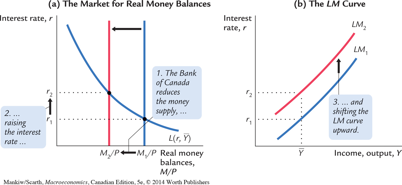
 , a reduction in the money supply raises the interest rate that equilibrates the money market. Therefore, the LM curve in panel (b) shifts upward.
336
In summary, the LM curve shows the combinations of the interest rate and the level of income that are consistent with equilibrium in the market for real money balances. The LM curve is drawn for a given supply of real money balances. Decreases in the supply of real money balances shift the LM curve upward. Increases in the supply of real money balances shift the LM curve downward.
A Quantity-Equation Interpretation of the LM Curve
When we first discussed aggregate demand and the short-run determination of income in Chapter 9, we derived the aggregate demand curve from the quantity theory of money. We described the money market with the quantity equation,
MV = PY,
and assumed that velocity V is constant. This assumption implies that, for any given price level P, the supply of money M by itself determines the level of income Y. Because the level of income does not depend on the interest rate, the quantity theory is equivalent to a vertical LM curve.
We can derive the more realistic upward-sloping LM curve from the quantity equation by relaxing the assumption that velocity is constant. The assumption of constant velocity is based on the assumption that the demand for real money balances depends only on the level of income. Yet, as we have noted in our discussion of the liquidity-preference model, the demand for real money balances also depends on the interest rate: a higher interest rate raises the cost of holding money and reduces money demand. When people respond to a higher interest rate by holding less money, each dollar they do hold must be used more often to support a given volume of transactions—that is, the velocity of money must increase. We can write this as
337
MV(r) = PY.
The velocity function V(r) indicates that velocity is positively related to the interest rate.
This form of the quantity equation yields an LM curve that slopes upward. Because an increase in the interest rate raises the velocity of money, it raises the level of income for any given money supply and price level. The LM curve expresses this positive relationship between the interest rate and income.
This equation also shows why changes in the money supply shift the LM curve. For any given interest rate and price level, the money supply and the level of income must move together. Thus, increases in the money supply shift the LM curve to the right, and decreases in the money supply shift the LM curve to the left.
Keep in mind that the quantity equation is merely another way to express the theory behind the LM curve. This quantity-theory interpretation of the LM curve is substantively the same as that provided by the theory of liquidity preference. In both cases, the LM curve represents a positive relationship between income and the interest rate that arises from the money market.
Finally, remember that the LM curve by itself does not determine either income Y or the interest rate r that will prevail in the economy. Like the IS curve, the LM curve is only a relationship between these two endogenous variables. To understand the economy’s overall equilibrium for a given price level, we must consider both equilibrium in the goods market and equilibrium in the money market. That is, we need to use the IS and LM curves together.