10.3 Conclusion: The Short-Run Equilibrium
We now have all the pieces of the IS–LM model. The two equations of this model are
| Y = C(Y – T) + I(r) + G | IS, |
| M/P = L(r, Y) | LM. |
The model takes fiscal policy, G and T, monetary policy M, and the price level P as exogenous. Given these exogenous variables, the IS curve provides the combinations of r and Y that satisfy the equation representing the goods market, and the LM curve provides the combinations of r and Y that satisfy the equation representing the money market. These two curves are shown together in Figure 10-14.
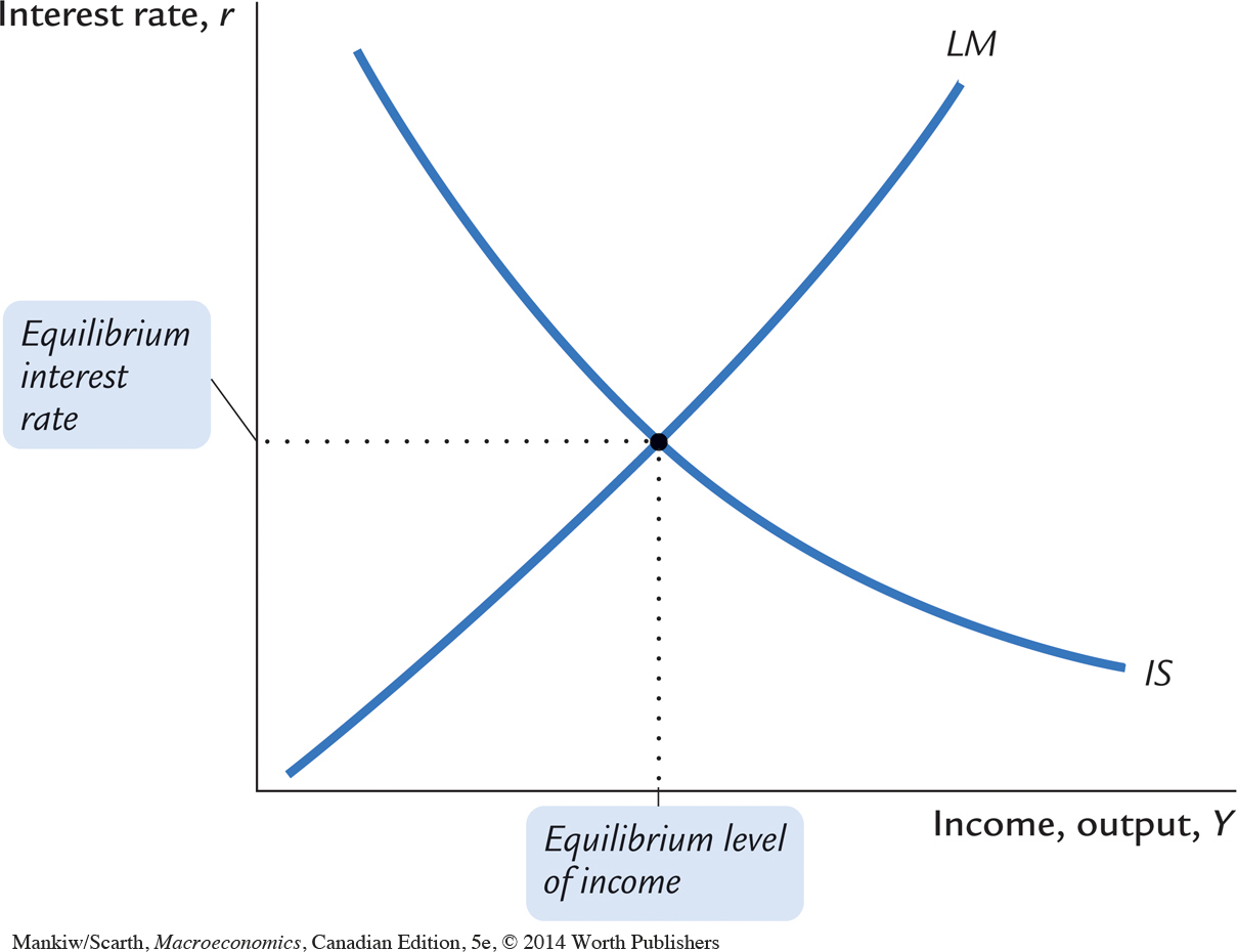
The equilibrium of the economy is the point at which the IS curve and the LM curve cross. This point gives the interest rate r and the level of income Y that satisfy conditions for equilibrium in both the goods market and the money market. In other words, at this intersection, actual expenditure equals planned expenditure, and the demand for real money balances equals the supply.
338
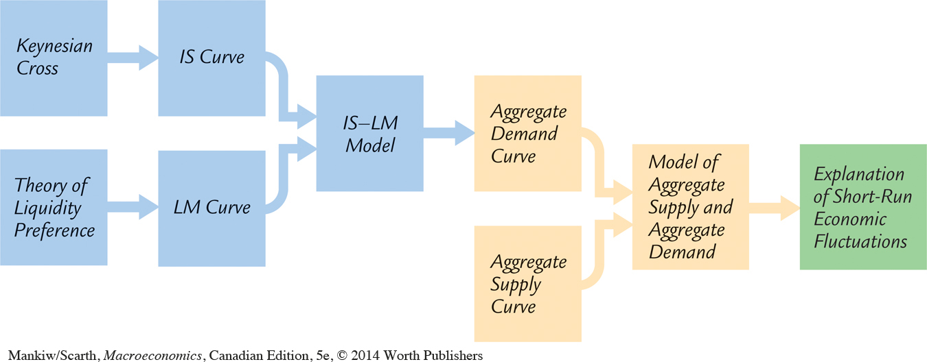
As we conclude this chapter, let’s recall that our ultimate goal in developing the IS–LM model is to analyze short-run fluctuations in economic activity. Figure 10-15 illustrates how the different pieces of our theory fit together. In this chapter we developed the Keynesian cross and the theory of liquidity preference as building blocks for the IS–LM model. As we see more fully in the next chapter, the IS–LM model helps explain the position and slope of the aggregate demand curve. The aggregate demand curve, in turn, is a piece of the model of aggregate supply and aggregate demand, which economists use to explain the short-run effects of policy changes and other events on national income.