11.1 Explaining Fluctuations With the IS–LM Model
344
The intersection of the IS curve and the LM curve determines the level of national income. When one of these curves shifts, the short-run equilibrium of the economy changes, and national income fluctuates. In this section we examine how changes in policy and shocks to the economy can cause these curves to shift.
How Fiscal Policy Shifts the IS Curve and Changes the Short-Run Equilibrium
We begin by examining how changes in fiscal policy (government purchases and taxes) alter the economy’s short-run equilibrium. Recall that changes in fiscal policy influence planned expenditure and thereby shift the IS curve. The IS–LM model shows how these shifts in the IS curve affect income and the interest rate.
Changes in Government Purchases Consider an increase in government purchases of ΔG. The government-purchases multiplier in the Keynesian cross tells us that, this change in fiscal policy raises the level of income at any given interest rate by ΔG/(1 − MPC). Therefore, as Figure 11-1 shows, the IS curve shifts to the right by this amount. The equilibrium of the economy moves from point A to point B. The increase in government purchases raises both income and the interest rate.
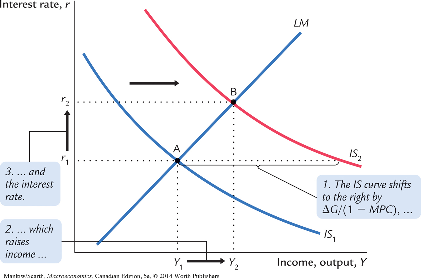
To understand fully what’s happening in Figure 11-1, it helps to keep in mind the building blocks for the IS–LM model from the preceding chapter—the Keynesian cross and the theory of liquidity preference. Here is the story. When the government increases its purchases of goods and services, the economy’s planned expenditure rises. The increase in planned expenditure stimulates the production of goods and services, which causes total income Y to rise. These effects should be familiar from the Keynesian cross.
Now consider the money market, as described by the theory of liquidity preference. Because the economy’s demand for money depends on income, the rise in total income increases the quantity of money demanded at every interest rate. The supply of money has not changed, however, so higher money demand causes the equilibrium interest rate r to rise.
The higher interest rate arising in the money market, in turn, has ramifications back in the goods market. When the interest rate rises, firms cut back on their investment plans. This fall in investment partially offsets the expansionary effect of the increase in government purchases. Thus, the increase in income in response to a fiscal expansion is smaller in the IS–LM model than it is in the Keynesian cross (where investment is assumed to be fixed). You can see this in Figure 11-1. The horizontal shift in the IS curve equals the rise in equilibrium income in the Keynesian cross. This amount is larger than the increase in equilibrium income here in the IS–LM model. The difference is explained by the crowding out of investment due to a higher interest rate.
345
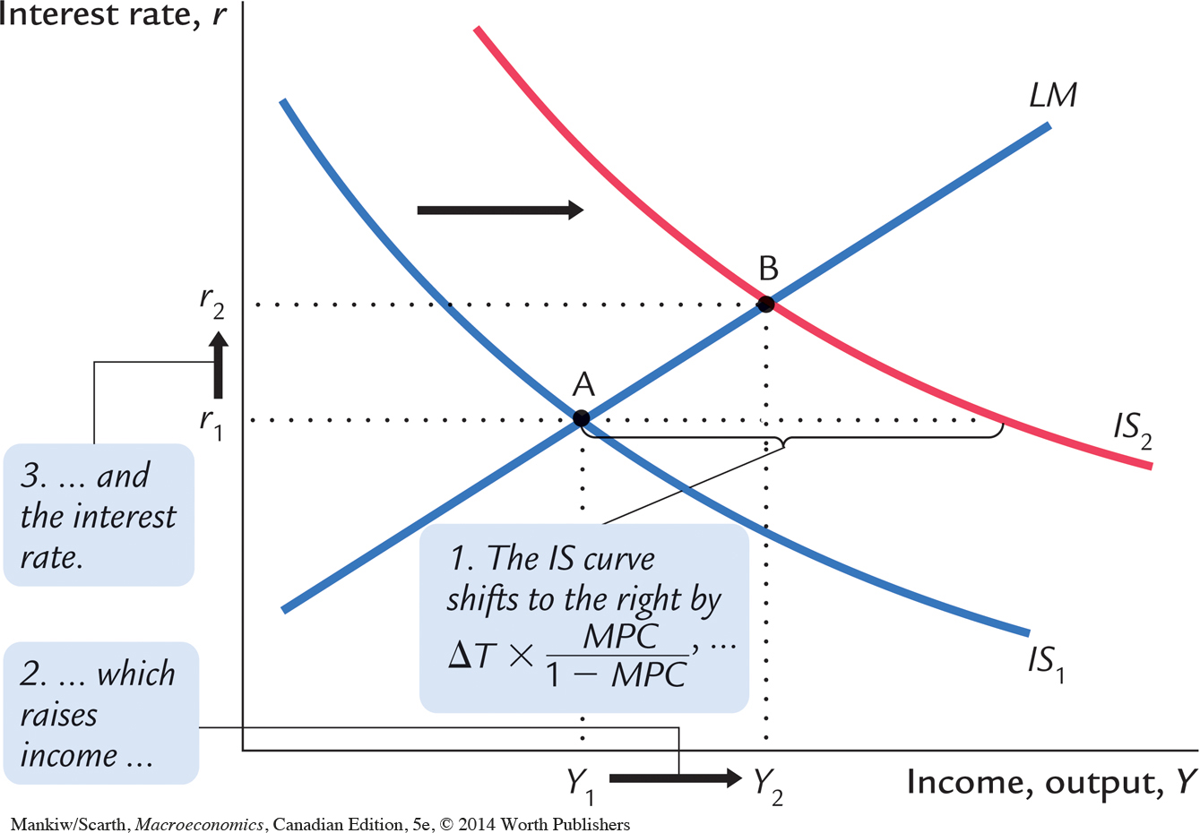
Changes in Taxes In the IS–LM model, changes in taxes affect the economy much the same as changes in government purchases do, except that taxes affect expenditure through consumption. Consider, for instance, a decrease in taxes of ΔT. The tax cut encourages consumers to spend more and, therefore, increases planned expenditure. The tax multiplier in the Keynesian cross tells us that this change in policy raises the level of income at any given interest rate by ΔT × MPC/(1 − MPC). Therefore, as Figure 11-2 illustrates, the IS curve shifts to the right by this amount. The equilibrium of the economy moves from point A to point B. The tax cut raises both income and the interest rate. Once again, because the higher interest rate depresses investment, the increase in income is smaller in the IS–LM model than it is in the Keynesian cross.
How Monetary Policy Shifts the LM Curve and Changes the Short-Run Equilibrium
We now examine the effects of monetary policy. Recall that a change in the money supply alters the interest rate that equilibrates the money market for any given level of income and, thus, shifts the LM curve. The IS–LM model shows how a shift in the LM curve affects income and the interest rate.
346
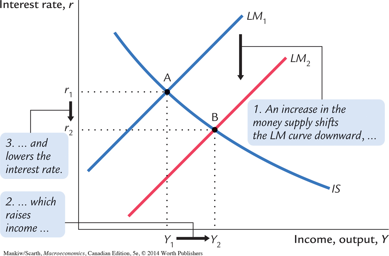
Consider an increase in the money supply. An increase in M leads to an increase in real money balances M/P, because the price level P is fixed in the short run. The theory of liquidity preference shows that for any given level of income, an increase in real money balances leads to a lower interest rate. Therefore, the LM curve shifts downward, as in Figure 11-3. The equilibrium moves from point A to point B. The increase in the money supply lowers the interest rate and raises the level of income.
347
Once again, to tell the story that explains the economy’s adjustment from point A to point B, we rely on the building blocks of the IS–LM model—the Keynesian cross and the theory of liquidity preference. This time, we begin with the money market, where the monetary policy action occurs. When the central bank increases the supply of money, people have more money than they want to hold at the prevailing interest rate. As a result, they start depositing this extra money in banks or use it to buy bonds. The interest rate r then falls until people are willing to hold all the extra money that the central bank has created; this brings the money market to a new equilibrium. The lower interest rate, in turn, has ramifications for the goods market. A lower interest rate stimulates planned investment, which increases planned expenditure, production, and income Y.
Thus, the IS–LM model shows that monetary policy influences income by changing the interest rate. This conclusion sheds light on our analysis of monetary policy in Chapter 9. In that chapter we showed that in the short run, when prices are sticky, an expansion in the money supply raises income. But we did not discuss how a monetary expansion induces greater spending on goods and services—a process that is called the monetary transmission mechanism. The IS–LM model shows an important part of that mechanism: an increase in the money supply lowers the interest rate, which stimulates investment and thereby expands the demand for goods and services. The next chapter shows that in open economies, the exchange rate also has a major role in the monetary transmission mechanism.
The Interaction Between Monetary and Fiscal Policy
When analyzing any change in monetary or fiscal policy, it is important to keep in mind that the policymakers who control these policy tools are aware of what the other policymakers are doing. A change in one policy, therefore, may influence the other, and this interdependence may alter the impact of a policy change.
For example, consider the federal government policy of eliminating the budget deficit during the 1990s by cutting government spending. What effect should this policy have on the economy? According to the IS–LM model, the answer depends on how the Bank of Canada responds to the spending cut.
Figure 11-4 shows three of the many possible outcomes that can follow from either a spending cut or a tax increase. In panel (a), the Bank of Canada holds the money supply constant. The spending cut shifts the IS curve to the left. Income falls (because lower spending reduces overall demand), and the interest rate falls (because lower income shifts downward the demand for money). The fall in income indicates that the fiscal policy causes a recession.
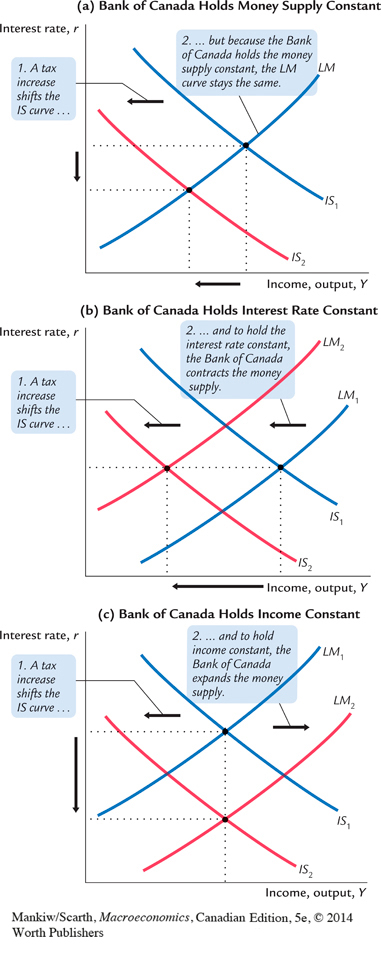
In panel (b), the Bank of Canada wants to hold the interest rate constant. In this case, when the spending cut shifts the IS curve to the left, the Bank of Canada must decrease the money supply to keep the interest rate at its original level. This fall in the money supply shifts the LM curve upward. The interest rate does not fall, but income falls by a larger amount than if the Bank of Canada had held the money supply constant. Whereas in panel (a) the lower interest rate stimulated investment and partially offset the contractionary effect of the spending cut, in panel (b) the Bank of Canada deepens the recession by keeping the interest rate high.
348
349
In panel (c), the Bank of Canada wants to prevent the spending cut from lowering income. It must, therefore, raise the money supply and shift the LM curve downward enough to offset the shift in the IS curve. In this case, the spending cut does not cause a recession, but it does cause a large fall in the interest rate. Although the level of income is not changed, the combination of a spending cut and a monetary expansion does change the allocation of the economy’s resources. The spending cut shrinks the government sector, while the lower interest rate stimulates investment. Income is not affected because these two effects exactly balance.
From this example we can see that the impact of a change in fiscal policy depends on the policy the Bank of Canada pursues—that is, on whether it holds the money supply, the interest rate, or the level of income constant. More generally, whenever analyzing a change in one policy, we must make an assumption about its effect on the other policy. What assumption is most appropriate depends on the case at hand and the many political considerations that lie behind economic policymaking.
Perhaps the most significant interaction between monetary and fiscal policy occurs in the case of a small open economy. In that case, the fundamental choice for monetary policy is whether to fix the exchange rate or to allow a flexible exchange rate. As we shall see in Chapter 12, this choice dramatically affects the power of fiscal policy. With a flexible exchange rate (and this has been Canada’s policy for years), the effect of fiscal policy on real GDP is very much blunted. This is good news for those who do not want spending cuts to raise unemployment very much, as was the case for our government in the 1990s, but this is bad news for those who want to use expansionary fiscal policy to create jobs, as was the case for our government in the recession of 2008–2009. We will explore these issues more fully in Chapter 12, after we have completed our development of the closed-economy model of aggregate demand.
CASE STUDY
Policy Analysis With Macroeconometric Models
The IS–LM model shows how monetary and fiscal policy influence the equilibrium level of income. The predictions of the model, however, are qualitative, not quantitative. The IS–LM model shows that increases in government purchases raise GDP and that increases in taxes lower GDP. But when economists analyze specific policy proposals, they need to know not just the direction of the effect but the size as well. For example, if the federal government cuts spending by $5 billion and if monetary policy is not altered, how much will GDP fall? To answer this question, economists need to go beyond the graphical representation of the IS–LM model.
Macroeconometric models of the economy provide one way to evaluate policy proposals. A macroeconometric model is a model that describes the economy quantitatively, rather than just qualitatively. Many of these models are essentially more complicated and more realistic versions of our IS–LM model. The economists who build macroeconometric models use historical data to estimate parameters such as the marginal propensity to consume, the sensitivity of investment to the interest rate, and the sensitivity of money demand to the interest rate. Once a model is built, economists can simulate the effects of alternative policies with the help of a computer.
350
It is interesting to note that estimates of Canada’s one-year government spending multiplier have changed substantially over the years. In the situation in which the Bank of Canada keeps the money supply constant, ΔY/ΔG was estimated to be 1.42 thirty years ago.1 This estimate meant that an increase in government spending of $1 billion was expected to raise overall GDP by $1.42 billion after one year. By 1986, multiplier estimates had fallen to 0.77.2 Finally, by the early 1990s, those using macroeconometric models were reporting government spending multipliers in the 0.50–0.67 range.3 This wide variation in estimates for ΔY/ΔG, all involving the same behaviour on the part of the Bank of Canada, implies a great deal of imprecision in the planning of fiscal policy. Why do the estimates of the power of fiscal policy keep shrinking as more research proceeds? Economists believe there are two reasons for this trend.
The first concerns the role of expectations on the part of households and firms. To see the importance of expectations, compare a temporary increase in government spending to a permanent one. The IS curve shifts out to the right in both cases, so interest rates rise, and this causes some cutback in the investment component of aggregate demand. But the size of this investment response depends on how permanent firms expect the rise in interest rates to be. If the increase in government spending is temporary, the rise in interest rates should be temporary as well, so firms’ investment spending is not curtailed to a very great extent. But if the increase in government spending is expected to be permanent, the rise in interest rates matters much more in firms’ long-range planning decisions, and there is a much bigger cutback in investment spending. Thus, the government spending multiplier is smaller when the change in spending is expected to last a long time.
You might think that, since changes in investment spending lag behind interest rate changes, this expectations issue cannot matter much for determining the multiplier value for a time horizon of just one year. But such a view amounts to assuming that individuals cannot see the interest changes coming. Anyone who understands the IS–LM model knows that permanently higher government spending raises interest rates. They also know that the value of existing financial assets (stocks and bonds) will fall when newly issued bonds promising higher yields are issued. No one wants to hold an asset with a low yield when better yields are expected. Thus, in an attempt to avoid a capital loss on existing financial assets, owners sell them the moment they expect a capital loss. That moment occurs as soon as they see a reason for interest rate increases—that is, just after the government spending increase has been announced (even before it is implemented). But if everyone tries to sell financial assets at the same time, the price of those assets drops quickly. As a result, the effective yield that a new purchaser can earn on them—the going rate of interest—rises immediately. The moral of the story is that when individuals react to well-informed expectations, their reactions have the effect of bringing the long-run implications of fiscal policy forward in time.
351
Over the last thirty years, economists have made major strides in their ability to model and simulate how individuals form expectations. Because of this development, the estimated econometric models have done a much better job of including the short-run implications of future government policies. This is a fundamental reason why the estimates of ΔY/ΔG have shrunk so much over time as research methods have improved.
The second explanation for the decrease in ΔY/ΔG estimates follows from increased globalization. With financial markets becoming ever more integrated throughout the world, there has developed an ever-expanding pool of “hot money.” These funds move into or out of a country like Canada the moment that the interest rate rises above or sinks below interest rate levels in other countries. This flow of funds dominates the trading in the foreign exchange markets, and so it results in large changes in exchange rates. We must wait until Chapter 12 to learn how these exchange-rate changes reduce the power of fiscal policy. But it is worth noting now that globalization has increased the size and speed of these exchange-rate effects, and so it is not surprising that estimated fiscal policy multipliers have shrunk over time.
It is interesting that, when introducing its “Action Plan” in the 2009 budget, our federal government based its deficit and job-creation plans on the assumption that the government spending multiplier would be 1.5. Was this estimate too high? Initial evidence suggested so, but perhaps not. The government did stress that their initiative was temporary, and it was the case that exchange-rate effects could be expected to be small when our central bank was keeping interest rates low and when our trading partners were taking similar initiatives simultaneously. In addition, the government tried to ensure low government spending on imports by concentrating on programs such as home renovation grants. 
Shocks in the IS–LM Model
Because the IS–LM model shows how national income is determined in the short run, we can use the model to examine how various economic disturbances affect income. So far we have seen how changes in fiscal policy shift the IS curve and how changes in monetary policy shift the LM curve. Similarly, we can group other disturbances into two categories: shocks to the IS curve and shocks to the LM curve.
Shocks to the IS curve are exogenous changes in the demand for goods and services. Some economists, including Keynes, have emphasized that such changes in demand can arise from investors’ animal spirits—exogenous and perhaps self-fulfilling waves of optimism and pessimism. For example, suppose that firms become pessimistic about the future of the economy and that this pessimism causes them to build fewer new factories. This reduction in the demand for investment goods causes a contractionary shift in the investment function: at every interest rate, firms want to invest less. The fall in investment reduces planned expenditure and shifts the IS curve to the left, reducing income and employment. This fall in equilibrium income in part validates the firms’ initial pessimism.

352
Shocks to the IS curve may also arise from changes in the demand for consumer goods. Suppose that consumer confidence rises, as people become less worried about losing their jobs. This induces consumers to save less for the future and consume more today. We can interpret this change as an upward shift in the consumption function. This shift in the consumption function increases planned expenditure and shifts the IS curve to the right, and this raises income.
FYI
What Is the Bank of Canada’s Policy Instrument—the Money Supply or the Interest Rate? And What Is Quantitative Easing?
Our analysis of monetary policy has been based on the assumption that the Bank of Canada influences the economy by controlling the money supply. By contrast, when you hear about Bank of Canada policy in the media, the policy instrument mentioned most often is the Bank Rate. It is the rate charged by the Bank of Canada when loaning reserves to the chartered banks, and it affects the overnight rate charged by the chartered banks when making overnight loans to each other. Which is the correct way of discussing policy? The answer is both.
For many years, the Bank of Canada has used the interest rate as its short-term policy instrument. This means that when the Bank decides on a target for the interest rate, the Bank’s bond traders are told to conduct the open-market operations necessary to hit that target. These open-market operations change the money supply and shift the LM curve so that the equilibrium interest rate (determined by the intersection of the IS and LM curves) equals the target interest rate that the Bank’s governing council has chosen.
As a result of this operating procedure, Bank of Canada policy is often discussed in terms of changing interest rates. Keep in mind, however, that behind these changes in interest rates are the necessary changes in the money supply. A newspaper might report, for instance, that “the Bank of Canada has lowered interest rates.” To be more precise, we can translate this statement as meaning “the Bank has instructed its bond traders to buy bonds in open-market operations and to pay for these bond purchases by issuing new money. This increases the money supply, shifts the LM curve to the right, and therefore reduces the equilibrium interest rate to hit a new lower target.”
Why has the Bank of Canada chosen to use an interest rate, rather than the money supply, as its short-term policy instrument? One possible answer is that shocks to the LM curve are more prevalent than shocks to the IS curve. If so, a policy of targeting the interest rate leads to greater macroeconomic stability than a policy of targeting the money supply. (Problem 7 at the end of this chapter asks you to analyze this issue.) Another possible answer is that interest rates are easier to measure than the money supply. As we saw in Chapter 4, the Bank of Canada has several different measures of money—M1, M2, and so on—which sometimes move in different directions. Rather than deciding which measure is best, the Bank of Canada avoids the question by using the interest rate as its short-term policy instrument. When the Bank of Canada imposes a value for the interest rate, the LM curve becomes unnecessary for determining the level of aggregate demand. We no longer need both the IS and LM relationships to jointly determine Y and r. Instead, we are in a situation in which the central bank sets r, the IS relationship determines aggregate demand, and the only role for the LM relationship is (residually) to indicate what value of the money supply was needed to deliver the target value of the rate of interest. We provide formal analyses of this no–LM-curve version of aggregate demand theory in the appendix to this chapter, and in Chapter 14.
353
Understanding the Bank of Canada’s short-term policy instrument became an even bigger challenge in 2009, after the Bank had lowered its overnight lending rate all the way to zero. Because no one will pay someone else to take money off his or her hands, there is a lower bound of zero on nominal interest rates. This same limit had been reached in North America during the Depression in the 1930s and during the prolonged slump in Japan during the 1990s. When that limit was reached in Canada, people questioned how it was then possible for the Bank of Canada to perform expansionary monetary policy. The short-term interest rate could not be lowered any more. The answer involved returning to a focus on the money supply instead of the interest rate, and arguing that the IS–LM model takes too narrow a view of the way money affects spending. In a broader view, households manage a portfolio of assets including money, financial claims, and consumer durables. When portfolios become out of balance—with too much money—households reallocate by acquiring more financial claims and durables. According to this view, money affects the goods market without having to “go through” interest rates, because there are direct money-to-goods reallocations within the portfolio. Consequently, the quantity of money has a direct effect on consumption, so a higher quantity of money shifts both the IS and LM curves to the right—not just the latter. “Quantitative Easing” refers to the Bank of Canada’s stimulation of aggregate demand in this way. In its Monetary Policy Report of April 2009, the Bank explained that it remains ready to buy longer term bonds as a way of implementing this strategy. Another way the bank has tried to stimulate demand when confronting the zero-lower-bound problem is by working on the public’s expectations. By promising to keep interest rates low even after the recovery from recession, the Bank hopes to create inflationary expectations, causing people to “buy now to beat the price increases.”
Shocks to the LM curve arise from exogenous changes in the demand for money. For example, suppose that the demand for money increases substantially, as it does when people become worried about the security of holding wealth in less liquid forms—a sensible worry if they expect a recession or a stock market crash. According to the theory of liquidity preference, when money demand rises, the interest rate necessary to equilibrate the money market is higher (for any given level of income and money supply). Hence, an increase in money demand shifts the LM curve upward, which tends to raise the interest rate and depress income—that is, to cause the very recession that individuals had feared.
In summary, several kinds of events can cause economic fluctuations by shifting the IS curve or the LM curve. Remember, however, that such fluctuations are not inevitable. Policymakers can try to use the tools of monetary and fiscal policy to offset exogenous shocks. If policymakers are sufficiently quick and skillful (admittedly, a big if), shocks to the IS or LM curves need not lead to fluctuations in income or employment.