354

We have been using the IS–LM model to explain national income in the short run when the price level is fixed. To see how the IS–LM model fits into the model of aggregate supply and aggregate demand introduced in Chapter 9, we now examine what happens in the IS–LM model if the price level is allowed to change. By examining the effects of a changing price level, we can finally deliver what was promised when we began our study of the IS–LM model: a theory to explain the position and slope of the aggregate demand curve.

Recall from Chapter 9 that the aggregate demand curve describes a relationship between the price level and the level of national income. In Chapter 9 this relationship was derived from the quantity theory of money. The analysis showed that for a given money supply, a higher price level implies a lower level of income. Increases in the money supply shift the aggregate demand curve to the right, and decreases in the money supply shift the aggregate demand curve to the left.

To understand the determinants of aggregate demand more fully, we now use the IS–LM model, rather than the quantity theory, to derive the aggregate demand curve. First, we use the IS–LM model to show why national income falls as the price level rises—that is, why the aggregate demand curve is downward sloping. Second, we examine what causes the aggregate demand curve to shift.

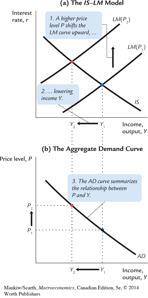
To explain why the aggregate demand curve slopes downward, we examine what happens in the IS–LM model when the price level changes. This is done in Figure 11-5. For any given money supply M, a higher price level P reduces the supply of real money balances M/P. A lower supply of real money balances shifts the LM curve upward, which raises the equilibrium interest rate and lowers the equilibrium level of income, as shown in panel (a). Here the price level rises from P₁ to P₂, and income falls from Y₁ to Y₂. The aggregate demand curve in panel (b) plots this negative relationship between national income and the price level. In other words, the aggregate demand curve shows the set of equilibrium points that arise in the IS–LM model as we vary the price level and see what happens to income.

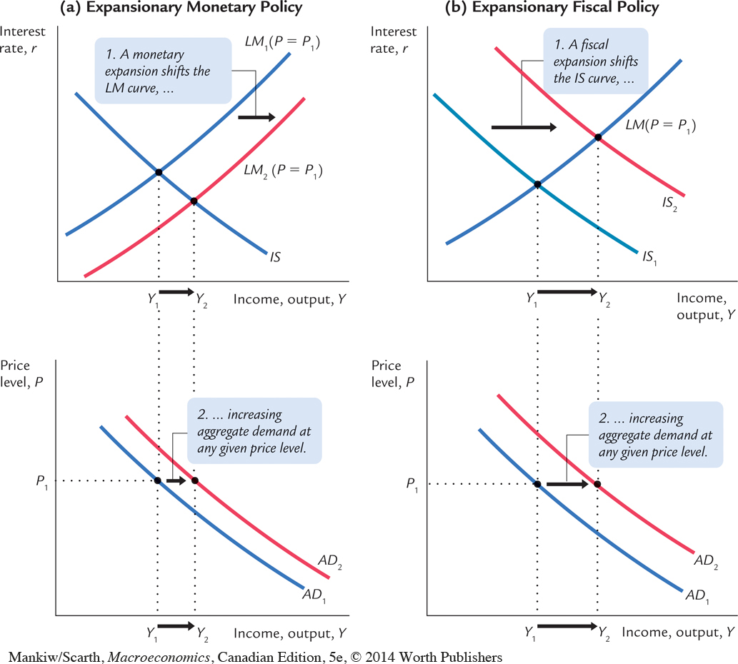
What causes the aggregate demand curve to shift? Because the aggregate demand curve summarizes the results from the IS–LM model, events that shift the IS curve or the LM curve (for a given price level) cause the aggregate demand curve to shift. For instance, an increase in the money supply raises income in the IS–LM model for any given price level; it thus shifts the aggregate demand curve to the right, as shown in panel (a) of Figure 11-6. Similarly, an increase in government purchases or a decrease in taxes raises income in the IS–LM model for a given price level; it also shifts the aggregate demand curve to the right, as shown in panel (b) of Figure 11-6. Conversely, a decrease in the money supply, a decrease in government purchases, or an increase in taxes lowers income in the IS–LM model and shifts the aggregate demand curve to the left. Anything that changes income in the IS–LM model other than a change in the price level causes a shift in the aggregate demand curve. The factors shifting aggregate demand include not only monetary and fiscal policy but also shocks to the goods market (the IS curve) and shocks to the money market (the LM curve).

355

We can summarize these results as follows: a change in income in the IS–LM model resulting from a change in the price level represents a movement along the aggregate demand curve. A change in income in the IS–LM model for a fixed price level represents a shift in the position of the aggregate demand curve.

356

The IS–LM model is designed to explain the economy in the short run when the price level is fixed. Yet, now that we have seen how a change in the price level influences the equilibrium in the IS–LM model, we can also use the model to describe the economy in the long run when the price level adjusts to ensure that the economy produces at its natural rate. By using the IS–LM model to describe the long run, we can show clearly how the Keynesian model of income determination differs from the classical model of Chapter 3.

357

Panel (a) of Figure 11-7 shows the three curves that are necessary for understanding the short-run and long-run equilibria: the IS curve, the LM curve, and the vertical line representing the natural level of output , which we label the full-employment output line. As explained in Chapter 3, this is the level of output that emerges when the market-clearing level of labour employment is inserted into the production function. Since neither the labour demand nor supply functions depend on the interest rate, this full-employment level of output is independent of r. That is why the full-employment output line is vertical in panel (a) of Figure 11-7. The LM curve is, as always, drawn for a fixed price level, P₁. The short-run equilibrium of the economy is point K, where the IS curve crosses the LM curve. Notice that in this short-run equilibrium, the economy’s income is less than its natural level.

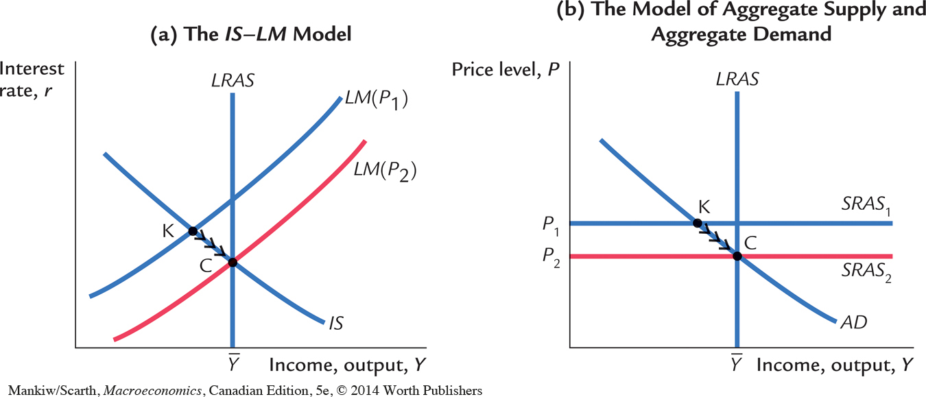
Panel (b) of Figure 11-7 shows the same situation in the diagram of aggregate supply and aggregate demand. At the price level P₁, the quantity of output demanded is below the natural level. In other words, at the existing price level, there is insufficient demand for goods and services to keep the economy producing at its potential.

In these two diagrams we can examine the short-run equilibrium at which the economy finds itself and the long-run equilibrium toward which the economy gravitates. Point K describes the short-run equilibrium, because it assumes that the price level is stuck at P₁. Eventually, the low demand for goods and services causes prices to fall, and the economy moves back toward its natural rate. When the price level reaches P₂, the economy is at point C, the long-run equilibrium. The diagram of aggregate supply and aggregate demand shows that at point C, the quantity of goods and services demanded equals the natural level of output. This long-run equilibrium is achieved in the IS–LM diagram by a shift in the LM curve: the fall in the price level raises real money balances and therefore shifts the LM curve to the right.

358

We can now see the key difference between the Keynesian and classical approaches to the determination of national income. The Keynesian assumption (represented by point K) is that the price level is stuck. Depending on monetary policy, fiscal policy, and the other determinants of aggregate demand, output may deviate from its natural level. The classical assumption (represented by point C) is that the price level is fully flexible. The price level adjusts to ensure that national income is always at its natural level.

To make the same point somewhat differently, we can think of the economy as being described by three equations. The first two are the IS and LM equations:

The IS equation describes the equilibrium in the goods market, and the LM equation describes the equilibrium in the money market. These two equations contain three endogenous variables: Y, P, and r. To complete the system, we need a third equation. The Keynesian approach completes the model with the assumption of fixed prices, so the Keynesian third equation is

P = P₁.

This assumption implies that the remaining two variables r and Y must adjust to satisfy the remaining two equations IS and LM. The classical approach completes the model with the assumption that output reaches its natural level, so the classical third equation is

This assumption implies that the remaining two variables r and P must adjust to satisfy the remaining two equations IS and LM. Thus, the classical approaches fixes output and allows the price level to adjust to satisfy the goods and money market equilibrium conditions, whereas the Keynesian approach fixes the price level and lets output move to satisfy the equilibrium conditions.

Which assumption is most appropriate? The answer depends on the time horizon. The classical assumption best describes the long run. Hence, our long-run analysis of national income in Chapter 3 and prices in Chapter 4 assumes that output equals the natural level. The Keynesian assumption best describes the short run. Therefore, our analysis of economic fluctuations relies on the assumption of a fixed price level.