11.3 The Great Depression
359
Now that we have developed the model of aggregate demand, let’s use it to address the question that originally motivated Keynes: what caused the Great Depression in the United States? For Canada, there is not such a puzzle. Since Canada exports such a large fraction of Canadian GDP to the United States, a depression in that country means a very big decrease in aggregate demand in Canada. Canada had no bank failures, so there is every reason to suspect that the loss in export sales was the dominant event. But what caused the Great Depression in the United States? Even today, more than half a century after the event, economists continue to debate the cause of this major economic downturn in the world’s most powerful economy. The Great Depression provides an extended case study to show how economists use the IS–LM model to analyze economic fluctuations.4
The Spending Hypothesis: Shocks to the IS Curve
Since the decline in U.S. income in the early 1930s coincided with falling interest rates, some economists have suggested that the cause of the decline was a contractionary shift in the IS curve. This view is sometimes called the spending hypothesis, because it places primary blame for the Depression on an exogenous fall in spending on goods and services. Economists have attempted to explain this decline in spending in several ways.
Some argue that a downward shift in the consumption function caused the contractionary shift in the IS curve. The stock market crash of 1929 may have been partly responsible for this decline in consumption. By reducing wealth and increasing uncertainty, the crash may have induced consumers to save more of their income.
Others explain the decline in spending by pointing to the large drop in investment in housing. Some economists believe that the residential investment boom of the 1920s was excessive, and that once this “overbuilding” became apparent, the demand for residential investment declined drastically. Another possible explanation for the fall in residential investment is the reduction in immigration in the 1930s: a more slowly growing population demands less new housing.
Once the Depression began, several events occurred that could have reduced spending further. First, the widespread bank failures in the United States (some 9,000 banks failed in the 1930–1933 period) may have reduced investment. Banks play the crucial role of getting the funds available for investment to those investors who can best use them. The closing of many banks in the early 1930s, with depositors losing their wealth, may have prevented some investors from getting the funds they needed and thus may have led to a further contractionary shift in the investment function.5
360
In addition, U.S. fiscal policy of the 1930s caused a contractionary shift in the IS curve. Politicians at that time were more concerned with balancing the budget than with using fiscal policy to stimulate the economy. The Revenue Act of 1932 increased various taxes, especially those falling on lower- and middle-income consumers.6 The Democratic platform of that year expressed concern about the budget deficit and advocated an “immediate and drastic reduction of governmental expenditures.” In the midst of historically high unemployment, policymakers searched for ways to raise taxes and reduce government spending.
There are, therefore, several ways to explain a contractionary shift in the IS curve. Keep in mind that these different views are not inconsistent with one another. There may be no single explanation for the decline in spending. It is possible that all of these changes coincided, and together they led to a major reduction in spending.
The Money Hypothesis: A Shock to the LM Curve
The U.S. money supply fell 25 percent from 1929 to 1933, during which time the unemployment rate rose from 3.2 percent to 25.2 percent. This fact provides the motivation and support for what is called the money hypothesis, which places primary blame for the Depression on the Federal Reserve for allowing the money supply to fall by such a large amount.7 The best known advocates of this interpretation are Milton Friedman and Anna Schwartz, who defend it in their treatise on U.S. monetary history. Friedman and Schwartz argue that contractions in the money supply have caused most economic downturns and that the Great Depression is a particularly vivid example.
Using the IS–LM model, we might interpret the money hypothesis as explaining the Depression by a contractionary shift in the LM curve. Seen in this way, however, the money hypothesis runs into two problems.
The first problem is the behaviour of real money balances. Monetary policy leads to a contractionary shift in the LM curve only if real money balances fall. Yet from 1929 to 1931, real money balances rose slightly, since the fall in the money supply was accompanied by an even greater fall in the price level. Although the monetary contraction may be responsible for the rise in unemployment from 1931 to 1933, when real money balances did fall, it probably should not be blamed for the initial downturn from 1929 to 1931.
361
The second problem for the money hypothesis is the behaviour of interest rates. If a contractionary shift in the LM curve triggered the Depression, we should have observed higher interest rates. Yet nominal interest rates fell continuously from 1929 to 1933.
These two reasons appear sufficient to reject the view that the Depression was instigated by a contractionary shift in the LM curve. But was the fall in the money stock irrelevant? Next, we turn to another mechanism through which monetary policy might have been responsible for the severity of the Depression—the deflation of the 1930s.
The Money Hypothesis Again: The Effects of Falling Prices
From 1929 to 1933 the U.S. price level fell 25 percent. Many economists blame this deflation for the severity of the Great Depression. They argue that the deflation may have turned what in 1931 was a typical economic downturn into an unprecedented period of high unemployment and depressed income. If correct, this argument gives new life to the money hypothesis. Since the falling money supply was, plausibly, responsible for the falling price level, it could have been responsible for the severity of the Depression. To evaluate this argument, we must discuss how changes in the price level affect income in the IS–LM model.
The Stabilizing Effects of Deflation In the IS–LM model we have developed so far, falling prices raise income. For any given supply of money M, a lower price level implies higher real money balances M/P. An increase in real money balances causes an expansionary shift in the LM curve, leading to higher income.
Another channel through which falling prices expand income is called the Pigou effect. Arthur Pigou, a prominent classical economist in the 1930s, pointed out that real money balances are part of households’ wealth. As prices fall and real money balances rise, consumers should feel wealthier and spend more. This increase in consumer spending should cause an expansionary shift in the IS curve, also leading to higher income.
These two reasons led some economists in the 1930s to believe that falling prices would help the economy restore itself to full employment. Yet other economists were less confident in the economy’s ability to correct itself. They pointed to other effects of falling prices, to which we now turn.
The Destabilizing Effects of Deflation Economists have proposed two theories to explain how falling prices could depress income rather than raise it. The first, called the debt-deflation theory, concerns the effects of unexpected falls in the price level. The second concerns the effects of expected deflation.
The debt-deflation theory begins with an observation that should be familiar from Chapter 4: unanticipated changes in the price level redistribute wealth between debtors and creditors. If a debtor owes a creditor $1,000, then the real amount of this debt is $1,000/P, where P is the price level. A fall in the price level raises the real amount of this debt—the amount of purchasing power the debtor must repay the creditor. Therefore, an unexpected deflation enriches creditors and impoverishes debtors.
362
The debt-deflation theory then posits that this redistribution of wealth affects spending on goods and services. In response to the redistribution from debtors to creditors, debtors spend less and creditors spend more. If these two groups have equal spending propensities, there is no aggregate impact. But it seems reasonable to assume that debtors have higher propensities to spend than creditors—perhaps that is why the debtors are in debt in the first place. In this case, debtors reduce their spending by more than creditors raise theirs. The net effect is a reduction in spending, a contractionary shift in the IS curve, and lower national income.
To understand how expected changes in prices can affect income, we need to add a new variable to the IS–LM model. Our discussion of the model so far has not distinguished between the nominal and real interest rates. Yet we know from previous chapters that investment depends on the real interest rate and that money demand depends on the nominal interest rate. If i is the nominal interest rate and Eπ is expected inflation, then the ex ante real interest rate r = i – Ep. We can now write the IS–LM model as
| Y = C(Y – T) + I(i – Eπ) + G | IS, |
| M/P = L(i, Y) | LM. |
Expected inflation enters as a variable in the IS curve. Thus, changes in expected inflation shift the IS curve, when it is drawn with the nominal interest rate on the vertical axis—as in Figure 11-8.
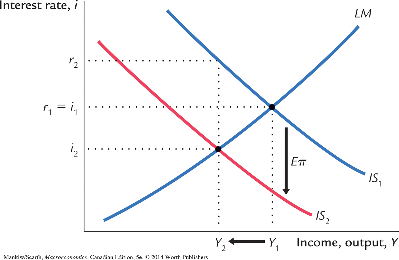
Let’s use this extended IS–LM model to examine how changes in expected inflation influence the level of income. We begin by assuming that everyone expects the price level to remain the same. In this case, there is no expected inflation (Eπ = 0), and these two equations produce the familiar IS–LM model. Now suppose that everyone suddenly expects that the price level will fall in the future, so that Eπ becomes negative. Figure 11-8 shows what happens. At any given nominal interest rate, the real interest rate is higher by the amount that Eπ has dropped. Thus, the IS curve shifts down by this amount, as investment spending is reduced. An expected deflation thus leads to a reduction in national income from Y1 to Y2. The nominal interest rate falls from i1 to i2, and since this is less than the drop in Eπ, the real interest rate rises from r1 to r2.
363
The logic behind this figure is straight—forward. When firms come to expect deflation, they become reluctant to borrow to buy investment goods because they believe they will have to repay these loans later in more valuable dollars. The fall in investment depresses planned expenditure, which in turn depresses income. The fall in income reduces the demand for money, and this reduces the nominal interest rate that equilibrates the money market. The nominal interest rate falls by less than the expected deflation, so the real interest rate rises.
Note that there is a common thread in these two reasons for destabilizing deflation. In both, falling prices depress national income by causing a contractionary shift in the IS curve. Because a deflation of the size observed from 1929 to 1933 is unlikely except in the presence of a major contraction in the money supply, these two explanations give some of the responsibility for the Depression—especially its severity—to the Federal Reserve in the United States. In other words, if falling prices are destabilizing, then a contraction in the money supply can lead to a fall in income, even without a decrease in real money balances or a rise in nominal interest rates.
Could the Depression Happen Again?
Economists study the Depression both because of its intrinsic interest as a major economic event and to provide guidance to policymakers so that it will not happen again. To state with confidence whether this event could recur, we would need to know why it happened. Because there is not yet agreement on the causes of the Great Depression, it is impossible to rule out with certainty another depression of this magnitude.
Yet most economists believe that the mistakes that led to the Great Depression are unlikely to be repeated. Central banks seem unlikely to allow the money supply to fall by one-fourth. Many economists believe that the deflation of the early 1930s was responsible for the depth and length of the Depression. And it seems likely that such a prolonged deflation was possible only in the presence of a falling money supply.
The fiscal-policy mistakes of the Depression are also unlikely to be repeated. Fiscal policy in the 1930s not only failed to help but actually further depressed aggregate demand. Few economists today would advocate such a rigid adherence to a balanced budget in the face of massive unemployment.
In addition, there are many institutions today that would help prevent the events of the 1930s from recurring. The system of deposit insurance (now available in both Canada and the United States, and discussed in Chapter 19) makes widespread bank failures less likely. Central banks are committed to providing price stability. The income tax causes an automatic reduction in taxes when income falls, which stabilizes the economy. Finally, economists know more today than they did in the 1930s. Our knowledge of how the economy works, limited as it still is, should help policymakers formulate better policies to combat such widespread unemployment.
364
CASE STUDY
The Financial Crisis and Economic Downturn of 2008 and 2009
In 2008, a financial crisis developed in the United States. Both the crisis and the ensuing recession spread to many countries. Several developments during this time were reminiscent of events during the 1930s; as a result, many observers feared a severe downturn in economic activity and a substantial rise in unemployment.
The story of the 2008 crisis begins a few years earlier with a substantial boom in the U.S. housing market. The boom had several origins. In part, it was fuelled by low interest rates, which made getting a mortgage less expensive for Americans and enabled them to buy higher priced homes. In addition, developments in the mortgage market made it easier for subprime borrowers—those borrowers with a higher risk of default based on their income and credit history—to get mortgages to buy homes. One of these developments was securitization, the process by which a financial institution (a mortgage originator) makes loans and then bundles them together into a variety of investment instruments called mortgage-backed securities. These mortgage-backed securities are then sold to other institutions (banks or insurance companies), which may not fully appreciate the risks they are taking. Some economists blame insufficient regulation for these high-risk loans. Others believe that, rather than too little regulation, the problem was the wrong kind of regulation: some government policies encouraged this high-risk lending to make the goal of home ownership more attainable for low-income families. Together, these forces drove up housing demand, and from 1995 to 2006, average housing prices in the United States more than doubled.
The high price of housing, however, proved unsustainable. From 2006 to 2008, housing prices fell about 20 percent nationwide in the United States. Such price fluctuations should not necessarily be a problem in a market economy. After all, price movements are how markets equilibrate supply and demand. Moreover, the price of housing in 2008 was merely a return to the level that had prevailed in 2004. But in this case, the price decline led to a series of problematic repercussions.
The first of these repercussions was a substantial rise in mortgage defaults and home foreclosures. During the housing boom, many homeowners had bought their homes with mostly borrowed money and minimal down payments. When housing prices declined, these homeowners were underwater: they owed more on their mortgages than their homes were worth. Many of these homeowners stopped paying their loans. The banks servicing the mortgages responded to these defaults by repossessing the houses in foreclosure procedures and then selling them. The banks wanted to recoup whatever they could. The increase in the number of homes for sale, however, exacerbated the downward spiral of housing prices.
365
A second repercussion was large losses at the various financial institutions that owned mortgage-backed securities. In essence, by borrowing large sums to buy high-risk mortgages, these companies had bet that housing prices would keep rising; when this bet turned bad, they found themselves at or near the point of bankruptcy. Even healthy banks stopped trusting one another and avoided interbank lending, because it was hard to discern which institution would be the next to go out of business. Due to these large losses at financial institutions and the widespread fear and distrust, the ability of the financial system to make loans even to creditworthy customers was impaired.
A third repercussion was a substantial rise in stock market volatility. Many companies rely on the financial system to get the resources they need for business expansion or to help them manage their short-term cash flows. With the financial system less able to perform its normal operations, the profitability of many companies was called into question. Because it was hard to know how bad things would get, stock market volatility reached levels not seen since the 1930s.
Higher stock market volatility, in turn, led to a fourth repercussion: a decline in consumer confidence. In the midst of all the uncertainty, households started putting off spending plans. Expenditures for durable goods in particular plummeted. As a result of all these events, the economy experienced a large contractionary shift in the IS curve.
The U.S. government responded vigorously as the crisis unfolded. First, the Fed cut its target for the federal funds rate from 5.25 percent in September 2007 to almost zero in December 2008. Second, in an even more unusual move in October 2008, the U.S. Congress appropriated $700 billion for the Treasury to use to rescue the financial system. Much of these funds were used for equity injections into banks. That is, the Treasury put funds into the banking system, and the banks could use these funds to make loans. In exchange for the funds, the U.S. government became a part owner of these banks, at least temporarily. The goal of the rescue (or “bailout,” as it was sometimes called) was to stem the financial crisis on Wall Street and prevent it from causing a depression on every other street in America. Finally, as noted in Chapter 10, when Barack Obama became president in January 2009, one of his first proposals was a major increase in government spending to expand aggregate demand.
Canada did not have a significant financial crisis in 2008, and several differences in institutional arrangements contributed to this much preferred outcome. First, Canada has a branch banking system with just a few banks operating throughout the country, and these banks are regulated in a coordinated fashion. The United States has a unit banking system with thousands of individual banks, many of them operating only within particular states. These individual banks do not have the advantage of pooling risks that larger banks do. Close to one-third of the banks failed in the United States during the first four years of the Depression in the 1930s, while none failed in Canada. This ongoing difference in industrial structure has continued to serve Canada well.
366
A second difference is that, until recently, the three main fields within our financial sector—banking, stock brokerage services, and insurance—were kept quite separate. This arrangement made it difficult for a “shadow” banking system to develop as it did in the United States. With shadow banking, institutions that are not covered by deposit insurance, such as stock brokerages, end up serving as people’s banks. This situation comes close to duplicating the fragility that existed before we introduced deposit insurance in the mid 1930s.
A third difference is the level of regulation. Canada’s banks must have $1 of underlying risk-free capital for every $18 of more risky assets they acquire by making loans. Under U.S. regulations before the crisis, each dollar of underlying capital permitted $25 of risky assets to be acquired. This freedom allowed U.S. banks to become overextended.
There is one final difference that made Canada less prone to a financial crisis. The crisis in the United States started in the housing/mortgage sector. Canadian institutional arrangements in this sector are quite different. For one thing, home ownership is not as heavily promoted north of the border. For example, mortgage payments are not deductible in the Canadian personal income tax system, and zero down payments are not permitted in Canada. Down payments of 20 percent are common here, and all mortgages with a loan-to-value ratio greater than 80 percent must be insured with a federal government agency (the Canada Mortgage and Housing Corporation), which applies strict standards.
Despite the fact that Canada avoided the U.S. financial crisis, Canadians still feared a serious domestic recession in 2008. This fear was based on the fact that we export such a large proportion of our GDP to the United States. A serious recession there means a big drop in Canadian exports, and consequently, a noticeable leftward shift in the position of Canada’s IS curve. For this reason, the Bank of Canada took action similar to the Fed’s, cutting the overnight lending rate all the way essentially to zero, and committing itself to a policy of quantitative easing if necessary (see the earlier FYI box in this chapter). Also, on the fiscal policy front, the federal government tabled a budget in 2009 that involved the biggest annual deficit in Canadian history. Both monetary policy and fiscal policy were being used to stimulate aggregate demand with the goal of keeping the recession from developing into anything like what we endured in the 1930s.
These policy initiatives were controversial. Some argued that the Bank of Canada’s readiness to pursue quantitative easing meant that the zero lower bound on nominal interest rates was not a problem, so the return to large fiscal deficits was ill advised. In the end, the government disagreed with this view. Readers who are interested in pursuing this debate in a way that integrates IS–LM theory and Canadian application can read a more detailed analysis provided elsewhere by one of the authors.8 
367
FYI
The Liquidity Trap
Short-term interest rates fell to zero throughout much of the western world in the 2008–2009 recession, just as they had in North America during the Great Depression in the 1930s and as they had during the prolonged slump in Japan during the 1990s.
Some economists describe this situation as a liquidity trap. According to the IS–LM model, expansionary monetary policy works by reducing interest rates and stimulating investment spending. But if interest rates have already fallen almost to zero, then perhaps monetary policy is no longer effective. Nominal interest rates cannot fall below zero: rather than making a loan at a negative nominal interest rate, a person would just hold cash. In this environment, expansionary monetary policy raises the supply of money, making the public more liquid, but because interest rates can’t fall any further, the extra liquidity might not have any effect. Aggregate demand, production, and employment may be “trapped” at low levels.
Other economists are skeptical about the relevance of liquidity traps and believe that central banks continue to have tools to expand the economy, even after its interest rate target hits zero. One possibility is that the central bank could raise inflation expectations by committing itself to future monetary expansion. Even if nominal interest rates cannot fall any further, higher expected inflation can lower real interest rates by making them negative, which would stimulate investment spending. A second possibility is that monetary expansion could cause the currency to lose value in the market for foreign currency exchange. This depreciation would make the nation’s goods cheaper abroad, stimulating export demand. This mechanism goes beyond the closed-economy IS–LM model we have used in this chapter, but it has merit in the open-economy version of the model developed in the next chapter. A third possibility is that the central bank could conduct expansionary open-market operations in a wider variety of financial instruments than it normally does. For example, it could buy mortgages and corporate debt and thereby lower the interest rates on these kinds of loans. The Federal Reserve in the United States actively pursued this last option during the downturn of 2008.
Is the liquidity trap something monetary policymakers need to worry about? Might the tools of monetary policy at times lose their power to influence the economy? There is no consensus about the answers. Skeptics say we shouldn’t worry about the liquidity trap. But others say the possibility of a liquidity trap argues for a target rate of inflation greater than zero. Under zero inflation, the real interest rate, like the nominal interest, can never fall below zero. But if the normal rate of inflation is, say, 3 percent, then the central bank can easily push the real interest rate to negative 3 percent by lowering the nominal interest rate toward zero. Thus, moderate inflation gives monetary policymakers more room to stimulate the economy when needed, reducing the risk of falling into a liquidity trap.9
A more detailed analysis of liquidity traps, which explains how aggregate supply and demand diagramatic analysis is affected, is available in the Appendix to this chapter.