372

APPENDIX

Aggregate Demand Theory Without the LM Curve

Some readers may find the two-quadrant diagrammatic derivation of the aggregate demand curve in Figure 11-5 confusing. The algebraic derivation presented in this appendix offers a second chance to understand this topic. A second purpose of this appendix is to eliminate the gap between news media reports that talk of the Bank of Canada “setting interest rates” and the discussion in Chapters 10 and 11 about the Bank setting the money supply. A third purpose of this appendix is to provide a more explicit discussion of how a liquidity trap can affect the power of monetary policy. For simplicity, as in Chapters 10 and 11, the algebraic treatment begins by abstracting from foreign trade. The small open economy case (in which foreign trade is central) is considered at the end of the appendix.

In the closed-economy setting, the relationships that define the components of aggregate demand are as follows:

Y = C + I + G

C = C* + c(Y – T)

I = I* + br

r = r* + a(P – P*)

The first equation states that the total of all goods produced, the GDP, must be purchased by households (C), firms (I), or the government (G). The household consumption function is the second equation (see Figure 10-2). C* stands for the vertical intercept in that figure, and c denotes the marginal propensity to consume (the slope of the line shown in Figure 10-2). As noted earlier, c is (realistically) assumed to be a positive fraction.

Firms’ investment spending on new plant and equipment depends inversely on the cost of borrowing. To capture this fact, we specify investment as an inverse function of the interest rate, r, in the third equation. I* is the intercept of this equation, and b is a positive parameter that defines the magnitude of the firms’ reaction to changes in the interest rate that they must pay on their loans.

Finally, the fourth equation defines the behaviour of the central bank. The bank’s goal is stable prices—that is, the bank wants to keep the price level, P, from either rising or falling. To pursue this goal, the bank adjusts the nation’s interest rate—so that the current value is above (or below) its long-run average value, r*—whenever the observed price level is above (or below) its target value, P*. The bank assumes that, by raising the interest rate, it will induce firms to cut back their spending. This reduction in aggregate demand is intended to induce firms to lower prices (and to bring the overall price index back to the bank’s target path). Parameter a defines the degree of aggressiveness that the central bank displays as it pursues this price stability objective.

373

When the four equations are combined (eliminating variables C, I, and r by substitution), the one remaining relationship is the equation that defines the nation’s aggregate demand function

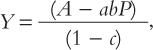
where A = (C* + I* + G – cT – br* + abP*). Since the slope of the aggregate demand curve (in price-output space) is rise/run = ΔP/ΔY, the expression that defines this slope is

This expression confirms that the slope of the demand curve is negative as long as the marginal propensity to consume is a fraction and as long as parameters a and b are both positive. The only one of these propositions that is in doubt is the one concerning the central bank parameter a. In some cases, the bank cannot manipulate the interest rate, and we must acknowledge this possibility by setting the bank’s reaction parameter to zero (a = 0) in some instances. The aggregate demand curve becomes vertical, not negatively sloped, in this situation, which we refer to as the “impotent” central bank case. We wish to explore both this and the opposite extreme possibility, which we call the “aggressive” central bank case.

With an aggressive central bank, monetary policy involves adjusting the interest rate so much and so quickly that the price level never departs from its target value. This approach means that the central bank’s reaction coefficient (parameter a) must be infinitely large. The equations just presented can be checked to verify that as parameter a tends to infinity, the equation of the aggregate demand relationship reduces to

P = P*

and the slope expression equals zero. So the aggregate demand relationship tends to a horizontal line at height P* as the central bank becomes ever more aggressive in targeting price stability. In the limit, the position of this line is not affected at all by changes in expenditure (changes in variables such as G and T), so fiscal policy is useless for affecting economic activity in this case. This is “bad news” if the government wants to create jobs with what is intended to be an “expansionary” fiscal policy. The reason this policy does not work is that, to avoid the upward pressure on the price level, the central bank raises the interest rate. This increase creates what is known as a “crowding out effect”: preexisting investment spending falls to make room for the higher public spending. But this outcome is “good news” if the government is cutting spending with a view to deficit reduction and it does not want to cause a recession in the process. In this case, the central bank response is lower interest rates, and this induces higher investment spending to take the place of the previously higher public spending. This analysis suggests that it was fortunate that Canada had a central bank that was actively committed to price stability when the fight against the deficit was proceeding during the 1990s.

374

The second extreme specification of monetary policy that we consider is one in which the central bank is unable to adjust the interest rate in the downward direction at all. This specification is relevant when the interest rate is already approximately zero, since it is impossible for nominal interest rates to become negative. (As explained at the end of Chapter 11, individuals always have the option of putting their money under their mattress). The equations just presented imply that the aggregate demand curve is vertical in this opposite extreme case.

We now consider how a situation that approaches each of these extremes can affect the ability of the economy to cure itself of a recession (Figure 11-9). There are two aggregate demand curves in this figure, and both intersect the short-run aggregate supply curve at point K. The price level (at value P₁) is too high to generate enough demand to secure full employment. The fairly flat demand curve is relevant when the central bank can and does adjust the interest rate fairly aggressively with a view to achieving price stability, while the much steeper demand curve is relevant when the central bank cannot adjust the interest rate significantly. In the first case, as prices fall, the economy moves from its Keynesian initial point (K) to the classical long-run outcome (point C) without too much deflation. But in the other case, deflation can continue indefinitely, without the economy ever getting back to full employment. As noted near the end of Chapter 11, a number of people feel that this “impotent central banker” case applied directly to the United States in the 1930s and to Japan in the 1990s. In both cases, the central bank could not lower interest rates (since yields were already essentially zero), and deflation did not eliminate the general stagnation of economic activity.

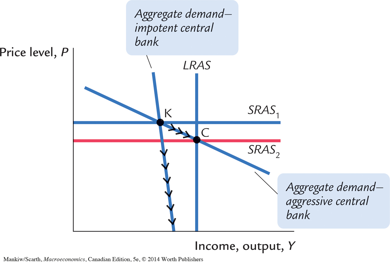
As already noted, Keynes called this outcome a “liquidity trap”: the central bank is trapped. It cannot decrease loan rates (by increasing the money supply), since households do not accept negative nominal interest rates. Keynes applied this analysis to the Great Depression of the 1930s. At that time, households had no desire to turn extra currency into stocks and bonds. They simply hoarded additional currency, and (as a result) central banks lost their ability to lower interest rates and affect aggregate demand. Consequently, Keynes called for expansionary fiscal policy during the Great Depression.

375

We now return to the algebraic derivation of the aggregate demand curve, but this time we introduce a slightly different reaction function on the part of the central bank—one that more closely matches the behaviour of the Bank of Canada. Readers may wish to postpone reading this section of the appendix until after they have studied Chapter 12. That chapter covers the version of aggregate demand theory suitable for a small economy that is integrated with the rest of the world in its trading relationship.

In an open economy, there is a net exports component of demand:

Y = C + I + G + NX.

We continue to assume that household consumption and firms’ investment spending depend on disposable income and the interest rate, respectively,

C = C* + c(Y – T),

I = I* – br.

We assume that net exports depend inversely on the relative price of domestic goods. From the point of view of foreigners, the cost of our goods depends on both the domestic currency price and the price of the Canadian dollar (the exchange rate, e). The following net export relationship embodies this assumption:

NX = X* – d(P + e).

In Chapter 18 we note that the Bank of Canada focuses on a weighted average of the interest rate and the exchange rate, known as the monetary conditions index (MCI). Defining the MCI as the Bank of Canada does,

MCI = r + (d/b)e,

and redefining the policy reaction function in the open-economy setting as

MCI = MCI* + a(P – P*),

we derive a summary aggregate demand relationship:

Y = C* + c(Y – T) + I* + G + X* – b[r + (d/b)e] – dP

= C* + c(Y – T) + I* + G + X* – b(MCI) – dP

= C* + c(Y – T) + I* + G + X* – b[MCI* + a(P – P*)] – dP

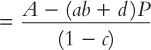
where A is now defined as C* – cT + I* + G + X* – b(MCI*) + abP*.

376

This summary expression for aggregate demand is similar to the one we have derived for the closed economy. As in that environment, we consider two polar cases. The first involves flexible exchange rates—a situation in which the central bank has no commitment to target any particular value for the exchange rate. As before, we assume that the central bank uses this independence to aggressively target domestic price stability. In this case, the central bank parameter a tends to infinity. The second situation involves a commitment to fix the exchange rate. With an ongoing obligation to buy and sell foreign exchange in whatever quantities dictated by market outcomes, the central bank has no independence to pursue any other policy objective. This impotence is imposed by setting central bank parameter a to zero. It can be readily verified that switching between these two cases (case 1—flexible exchange rates with the central bank imposing price stability and case 2—fixed exchange rates) has a big effect on the nature of the country’s aggregate demand curve. We consider each case in turn.

With flexible exchange rates, the aggregate demand equation tends toward a horizontal line defined by P = P* as the central bank pursues price stability ever more aggressively. Since variables such as G, T, and X* drop out of the equation, aggregate demand is completely unaffected by domestic fiscal policy or developments in the rest of the world. This is “bad news” for the government if it wants to use changes in its budget to conduct a stabilization policy. However, it is “good news” from the point of view that the economy is insulated from shocks that occur in the rest of the world (such as a recession in the United States, which would cause a drop in Canadian exports). The intuition behind these results is provided in Chapter 12.

With fixed exchange rates, the central bank is unable to target the price level. But since the slope of the aggregate demand curve (equal to −(1 − c)/d)) remains negative, Keynes’s liquidity trap concern represents a less serious problem for a small open economy. A recession can end via a change in the exchange rate, so a change in the interest rate is not necessary.

This result suggests that a flexible exchange rate is a shock absorber; when aggregate demand falls, a depreciating Canadian dollar provides one way for demand to increase again, and this degree of freedom is lost if the exchange rate is fixed. Figure 11-9 can be used to illustrate this feature of a flexible exchange rate policy, if we reinterpret the two aggregate demand curves. The steep curve must be relabelled “aggregate demand with a fixed exchange rate” and the flatter demand curve must be relabelled “aggregate demand with a flexible exchange rate.” Then we assume that the same loss in demand has pushed both the fixed-exchange-rate economy and the flexible-exchange-rate economy to point K in the short run. According to Figure 11-9, the deflation that occurs naturally when there is insufficient aggregate demand will eliminate the recession fairly readily under flexible exchange rates, but it will not do so with a fixed exchange rate. This analysis leads officials at the Bank of Canada to argue that Canada is well served by having a currency that is independent from the U.S. dollar (via a flexible exchange rate policy).