12.1 The Mundell–Fleming Model
In this section we build the Mundell–Fleming model, and in the following sections we use the model to examine the impact of various policies. As you will see, the Mundell–Fleming model is built from components we have used in previous chapters. But these pieces are put together in a new way to address a new set of questions.
Components of the Model
379
The Mundell–Fleming model is made up of components that should be familiar. We begin by simply stating the three equations that make up the model. They are
| Y = C(Y – T) + I(r) + G + NX(e) | IS, |
| M/P = L(r, Y) | LM, |
| r = r* |
Before putting these equations together to make a short-run model of a small open economy, let’s review each of them in turn.
The first equation describes the goods market. It states that aggregate supply Y is equal to aggregate demand—the sum of consumption C, investment I, government purchases G, and net exports NX. Consumption depends positively on disposable income Y – T. Investment depends negatively on the interest rate r. Net exports depend negatively on the exchange rate e.
Recall that we define the exchange rate e as the amount of foreign currency per unit of domestic currency—for example, e might be $0.90 (U.S.) per Canadian dollar. For the purposes of the Mundell–Fleming model, we do not need to distinguish between the real and nominal exchange rates. In Chapter 5 we related net exports to the real exchange rate є, which equals eP/P*, where P is the domestic price level and P* is the foreign price level. Because the Mundell–Fleming model assumes that prices are fixed, changes in the real exchange rate are proportional to changes in the nominal exchange rate. That is, when the nominal exchange rate rises, foreign goods become less expensive compared to domestic goods, which depresses exports and stimulates imports.
The second equation describes the money market. It states that the supply of real money balances, M/P, equals the demand, L(r, Y). The demand for real balances depends negatively on the interest rate and positively on overall output. As long as we have a floating exchange rate, the money supply M is an exogenous variable controlled by the central bank. Like the IS–LM model, the Mundell–Fleming model takes the price level P as an exogenous variable, so there is no difference between nominal and real interest rates.
The third equation states that the world interest rate r* determines the interest rate in this economy. This equation holds because we are examining a small open economy. That is, the economy is sufficiently small relative to the world economy that it can borrow or lend as much as it wants in world financial markets without affecting the world interest rate.
Although the idea of perfect capital mobility is expressed mathematically with a simple equation, it is important not to lose sight of the sophisticated process that this equation represents. Imagine that some event were to occur that would normally raise the interest rate (such as a decline in domestic saving). In a small open economy, the domestic interest rate might rise by a little bit for a short time, but as soon as it did, foreigners would see the higher interest rate and start lending to this country (by, for instance, buying this country’s bonds). The capital inflow would drive the domestic interest rate back toward r*. Similarly, if any event were ever to start driving the domestic interest rate downward, capital would flow out of the country to earn a higher return abroad, and this capital outflow would pull the domestic interest rate back upward toward r*. Hence, the r = r* equation represents the assumption that the international flow of capital is sufficiently rapid and large as to keep the domestic interest rate equal to the world interest rate.
380
It should be recalled from our discussion in Chapter 5 (in particular from Figure 5-2) that there are deviations of the Canadian interest rate from the world interest rate. One form of departure is a risk premium that depends on such factors as international concern about political instability in Canada (for example, Quebec separation). We consider risk premiums later on in this chapter, but initially they are ignored. The second reason for departures from the r = r* condition is that it takes some time for international lenders to react to yield differentials (and in doing so, to eliminate them). Thus, we view r = r* as representing full equilibrium, and we can consider temporary deviations from this full equilibrium while discussing the time sequence involved in the Mundell–Fleming model.
These three equations fully describe the Mundell–Fleming model. Our job is to examine the implications of these equations for short-run fluctuations in a small open economy. If you do not understand the equations, you should review Chapters 5 and 10 before continuing.
The Model on a Y–r Graph
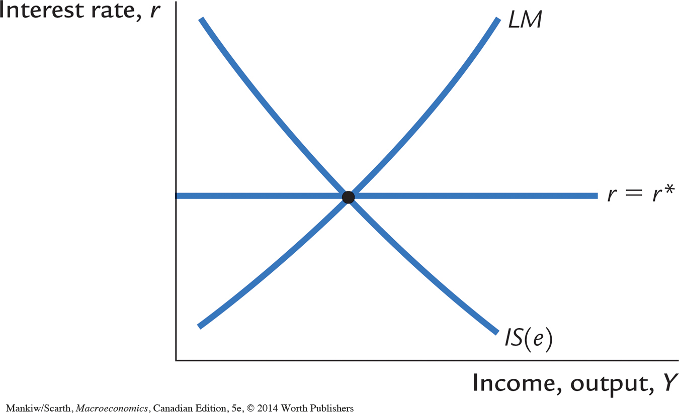
One way to depict the Mundell–Fleming model is to use a graph in which income Y is on the horizontal axis and the interest rate r is on the vertical axis. This presentation is comparable to our analysis of the closed economy in the IS–LM model. As Figure 12-1 shows, the IS curve slopes downward, and the LM curve slopes upward. New in this graph is the horizontal line representing the world interest rate.
381
Two features of this graph deserve special attention. First, because the exchange rate influences the demand for goods, the IS curve is drawn for a given value of the exchange rate (say, $0.90 (U.S.) per Canadian dollar). An increase in the exchange rate (say, to $0.95 (U.S.) per Canadian dollar) makes Canadian goods more expensive for foreigners to purchase, relative to foreign goods, which reduces net exports. Hence, an increase in the value of our dollar shifts the IS curve to the left. To remind us that the position of the IS curve depends on the exchange rate, the IS curve is labelled IS(e).
Second, the three curves in Figure 12-1 all intersect at the same point. This might seem an unlikely coincidence. But, in fact, the exchange rate adjusts to ensure that all three curves pass through the same point.
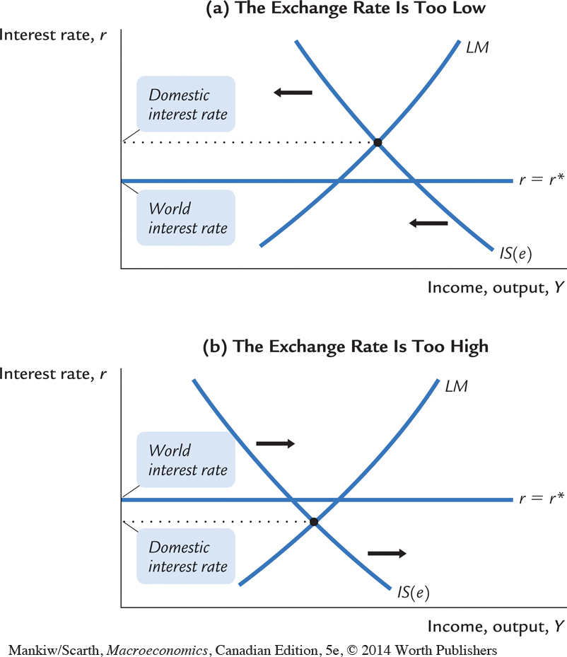
To see why all three curves must intersect at a single point, let’s imagine a hypothetical situation in which they did not, as in panel (a) of Figure 12-2. Here, the domestic interest rate—the point where the IS and LM curves intersect—would be higher than the world interest rate. Since Canada would be offering a higher rate of return than is available in world financial markets, investors from around the world would want to buy Canadian financial assets. But first these foreign investors must convert their funds into dollars. In the process, they would bid up the value of the Canadian dollar. This rise in the exchange rate would shift the IS curve downward until the domestic interest rate equaled the world interest rate.
382
Alternatively, imagine that the IS and LM curves intersect at a point where the domestic interest rate is below the world interest rate, as in panel (b) of Figure 12-2. Since Canada would be offering a lower rate of return, investors would want to invest in world financial markets. But, to be able to buy foreign financial assets, they must convert their Canadian dollars into foreign currency. In the process of doing so, they would depress the value of the Canadian dollar. The fall in the exchange rate would stimulate Canadian export sales and so shift the IS curve upward until the domestic interest rate equaled the world interest rate.
To sum up, the equilibrium in this graph is found where the LM curve crosses the line representing the world interest rate. The exchange rate then adjusts and shifts the IS curve so that the IS curve crosses this point as well.
The Model on a Y–e Graph
The second way to depict the model is to use a graph in which income is on the horizontal axis and the exchange rate is on the vertical axis, as in Figure 12-3. This graph is drawn holding the interest rate constant at the world interest rate. The two equations in this figure are
| Y = C(Y – T) + I(r*) + G + NX(e) | IS*, |
| M/P = L(r*, Y) | LM* |
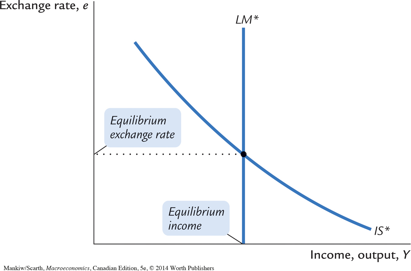
We label these curves IS* and LM* to remind us that we are holding the interest rate constant at the world interest rate r*. The equilibrium of the economy is found where the IS* curve and the LM* curve intersect. This intersection determines the exchange rate and the level of income.
383
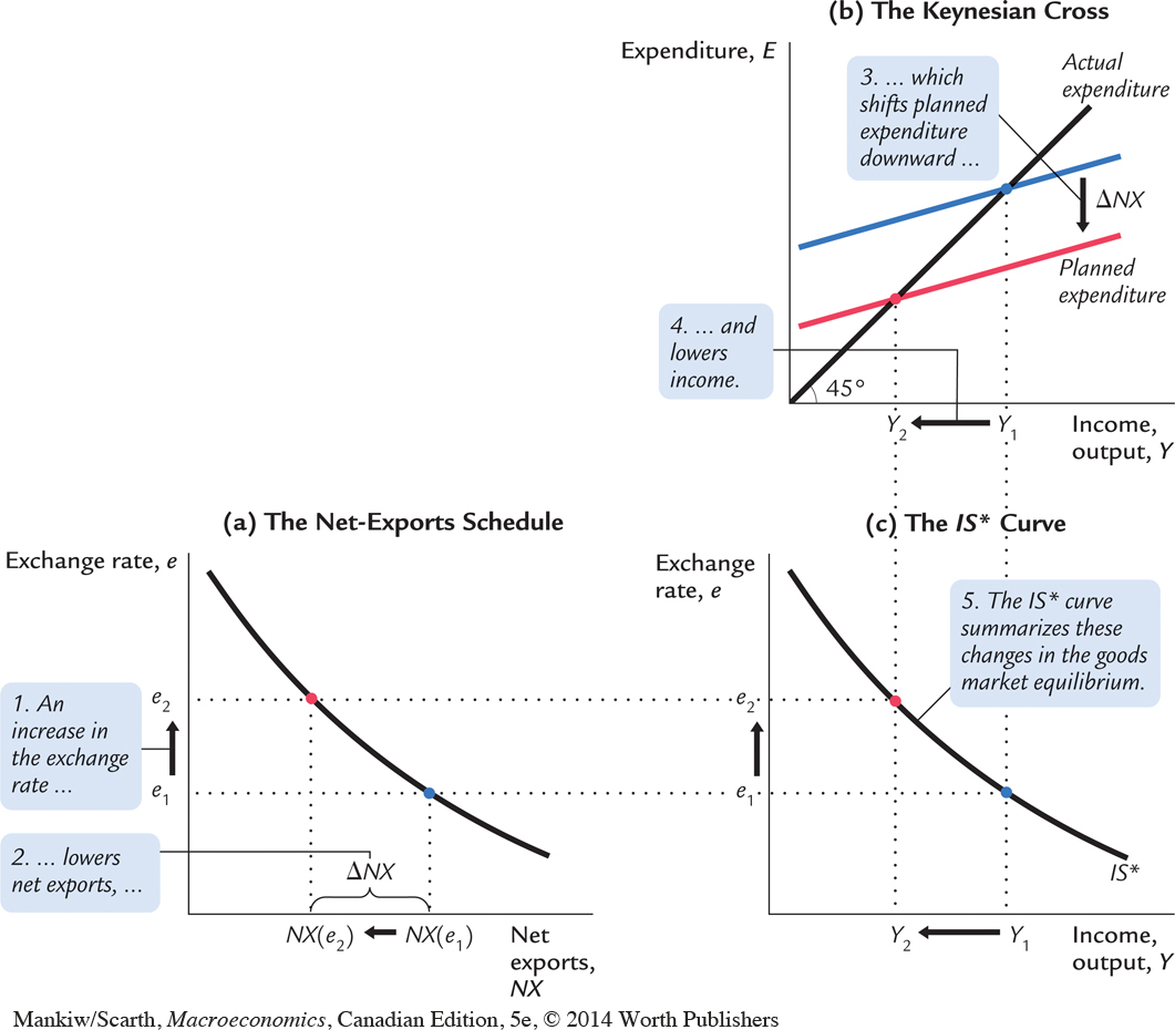
The IS* curve slopes downward because a higher exchange rate lowers net exports and thus lowers aggregate income. To show how this works, Figure 12-4 combines the net-exports schedule and the Keynesian-cross diagram to derive the IS* curve. An increase in the Canadian dollar from e1 to e2 lowers net exports from NX(e1) to NX(e2). The reduction in net exports reduces planned expenditure and thus lowers income. Just as the standard IS curve combines the investment schedule and the Keynesian cross, the IS* curve combines the net-exports schedule and the Keynesian cross.
384
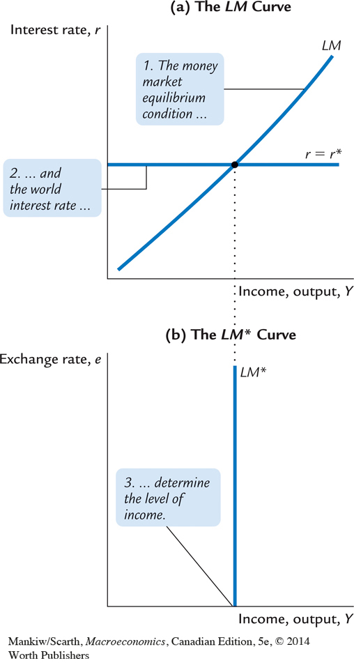
The LM* curve is vertical because the exchange rate does not enter into the LM* equation. Given the world interest rate, the LM* equation determines aggregate income, regardless of the exchange rate. Figure 12-5 shows how the LM* curve arises from the world interest rate and the LM curve, which relates the interest rate and income.
We can now use the IS*–LM* diagram (Figure 12-3). The equilibrium for the economy is found where the IS* curve and the LM* curve intersect. This intersection shows the exchange rate and the level of income at which the goods market and the money market are both in equilibrium. With this diagram, we can use the Mundell–Fleming model to show how aggregate income Y and the Canadian dollar e respond to changes in policy.