12.2 The Small Open Economy Under Floating Exchange Rates
385
Before analyzing the impact of policies in an open economy, we must specify the international monetary system in which the country has chosen to operate. That is, we must consider how people engaged in international trade and finance can convert the currency of one country into the currency of another.
We start with the system relevant for most major economies today: floating exchange rates. Under a system of floating, or flexible, exchange rates, the exchange rate is set by market forces and is allowed to fluctuate in response to changing economic conditions. In this case, the exchange rate e adjusts to achieve simultaneous equilibrium in the goods market and the money market. When something happens to change that equilibrium, the exchange rate is allowed to move to a new equilibrium value, since the central bank does not intervene in the foreign exchange market.
Let’s now consider three policies that can change the equilibrium: fiscal policy, monetary policy, and trade policy. Our goal is to use the Mundell–Fleming model to show the impact of policy changes and to understand the economic forces at work as the economy moves from one equilibrium to another.
Fiscal Policy
Suppose that the government stimulates domestic spending by increasing government purchases or by cutting taxes. Because such expansionary fiscal policy increases planned expenditure, it shifts the IS* curve to the right, as in Figure 12-6. As a result, the exchange rate appreciates, while the level of income remains the same.
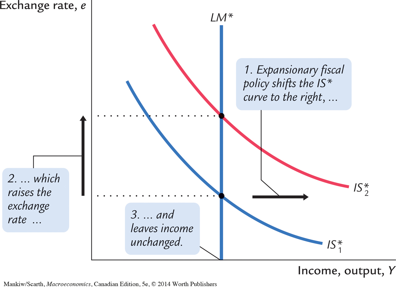
Notice that fiscal policy has very different effects in a small open economy than it does in a closed economy. In the closed-economy IS–LM model, a fiscal expansion raises income, whereas in a small open economy with a floating exchange rate and, as the interest rate rises, because higher income increases the demand for money. That is not possible in a small open economy because, as soon as the interest rate starts to rise above the world interest rate r*, capital quickly flows in from abroad to take advantage of the higher return. This capital inflow not only pushes the interest rate back to r* but it also has another effect: because foreign investors need to buy the domestic currency to invest in the domestic economy, the capital inflow increases the demand for the domestic currency in the market for foreign-currency exchange, bidding up the value of the domestic currency. The appreciation of the domestic currency makes domestic goods expensive relative to foreign goods, reducing net exports. The fall in net exports exactly offsets the effects of the expansionary fiscal policy on income. Thus, in a small open economy with a floating exchange rate, a fiscal expansion leaves income at the same level.
386
Why is the fall in net exports so great as to render fiscal policy completely powerless to influence income? To answer this question, consider the equation that describes the money market:
M/P = L(r, Y).
In both closed and open economies, the quantity of real money balances supplied M/P is fixed by the central bank (which sets M) and the assumption of sticky prices (which fixes P). The quantity demanded (determined by r and Y) must equal this fixed supply. In a closed economy, a fiscal expansion causes the equilibrium interest rate to rise. This increase in the interest rate (which reduces the quantity of money demanded) implies an increase in equilibrium income (which raises the quantity of money demanded). These two effects together maintain equilibrium in the money market. By contrast, in a small open economy, r is fixed at r*, so there is only one level of income that can satisfy this equation, and this level of income does not change when fiscal policy changes. Thus, when the government increases spending or cuts taxes, the appreciation of the exchange rate and the fall in net exports must be exactly large enough to offset fully the normal expansionary effect of the policy on income.
Monetary Policy
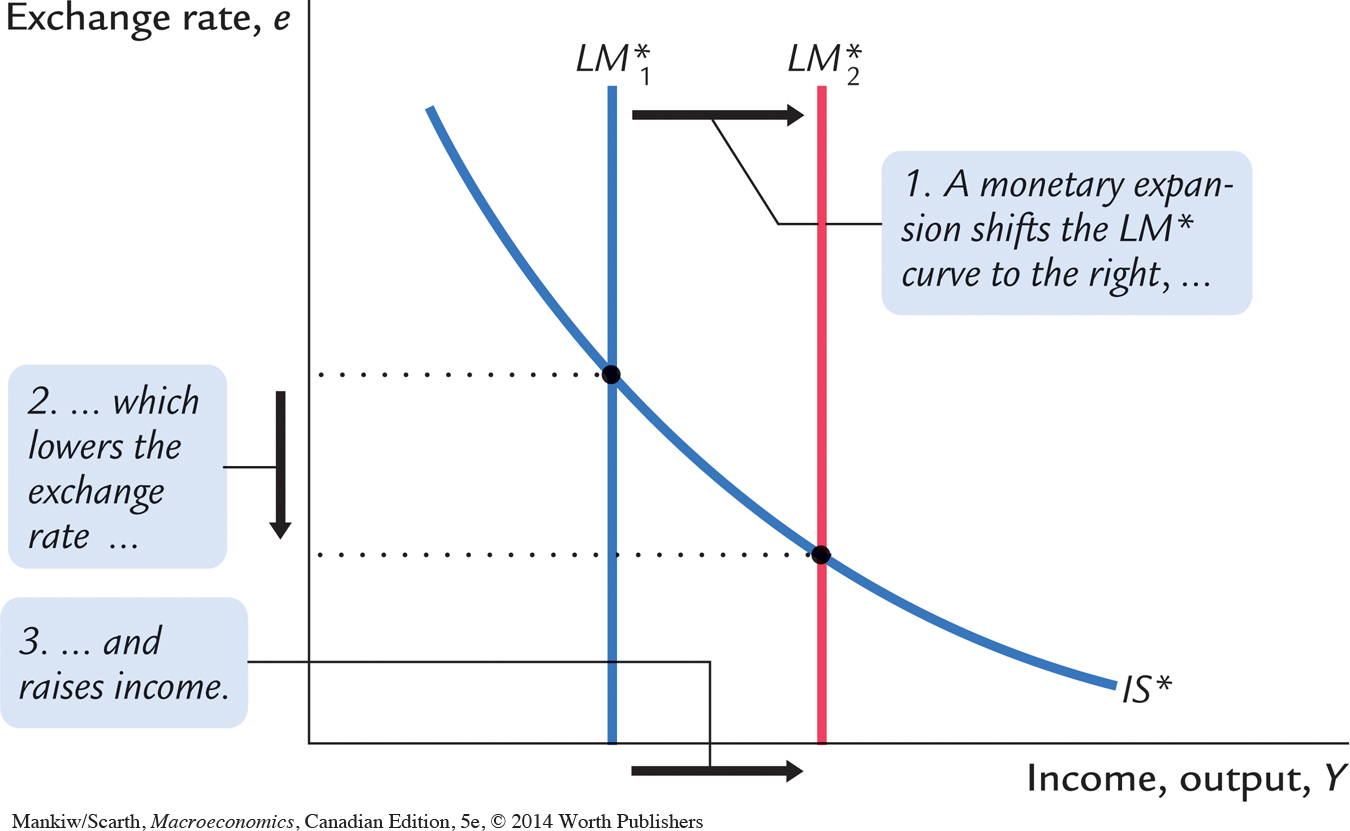
Suppose now that the Bank of Canada increases the money supply. Because the price level is assumed to be fixed, the increase in the money supply means an increase in real balances. The increase in real balances shifts the LM* curve to the right, as in Figure 12-7. Hence, an increase in the money supply raises income and lowers the exchange rate.
387
Although monetary policy influences income in an open economy, as it does in a closed economy, the monetary transmission mechanism is different. Recall that in a closed economy an increase in the money supply increases spending because it lowers the interest rate and stimulates investment. In a small open economy, this channel of monetary transmission is not available because the interest rate is fixed by the world interest rate. So how does monetary policy influence spending? To answer this question, once again we need to think about the international flow of capital and its implications for the domestic economy.
The interest rate and the exchange are again the key variables. As soon as an increase in the money supply puts downward pressure on the domestic interest rate, capital flows out of the economy, as investors seek a higher return elsewhere. This capital outflow prevents the domestic interest rate from falling below the world interest rate r*. It also has another effect: because investing abroad requires converting domestic currency into foreign currency, the capital outflow increases the supply of the domestic currency in the market for foreign-currency exchange, causing the domestic currrency to fall in value. This depreciation in the exchange rate makes domestic goods inexpensive relative to foreign goods and, thereby, stimulates net exports and overall demand. Hence, in a small open economy, monetary policy influences income by altering the exchange rate rather than the interest rate.
CASE STUDY
Tight Monetary Policy Combined With Loose Fiscal Policy
During the late 1980s, Canada experienced a combination of tight monetary policy and loose fiscal policy. The Governor of the Bank of Canada, John Crow, was committed to bringing inflation down, and his success earned him quite a reputation among the world central bankers. But both the federal and provincial governments were following an expansionary fiscal policy; their expenditures were far in excess of their tax revenues. Government deficits were increasing at record rates.
388
The Mundell–Fleming model predicts that both policies would raise the value of the Canadian dollar, and, indeed, Canadian currency did rise. In 1985 1 Canadian dollar could be purchased for $0.71 (U.S.), and by 1991 its price had risen to $0.89 (U.S.). This rise in the Canadian dollar made imported goods less expensive, and it made Canadian industries that compete against these foreign sellers less competitive. It is no wonder that this period witnessed a dramatic increase in “cross-border shopping by Canadians.”
Many analysts have noted that it was unfortunate that Canada’s monetary-fiscal policy mix during this period was so counterproductive for Canadian firms’ gaining a foothold in the U.S. markets following the signing of the Free Trade Agreement in January 1989. At the very time Canadian producers were becoming more competitive in the United States, because of the removal of U.S. tariffs on Canadian exports, these firms were becoming less competitive because of the dramatic rise in the value of the Canadian dollar.
Canada witnessed a similar mix of tight money and loose fiscal policy some 30 years earlier. John Diefenbaker, Canada’s prime minister at the time, was trying to reduce unemployment during the worst postwar recession up to that point by raising government spending and cutting taxes (the same set of policies used by our government as this book goes to press—as officials struggle to limit the 2009 recession). But James Coyne, the Governor of the Bank of Canada during Diefenbaker’s time, was focused exclusively on keeping the inflation rate close to zero. Thus, Coyne refused to print any new currency to help finance the government’s deficit. The result was just what the Mundell–Fleming model predicts. Funds flowed into Canada, and the value of the Canadian dollar increased dramatically. This put a further profit squeeze on Canadian exporting firms, so that as rapidly as the government was creating jobs in the government sector, the rising Canadian dollar was destroying jobs in the exporting and import-competing sectors.
The dispute between the government and the Bank of Canada Governor became so bitter during the Coyne affair that the Bank of Canada Act was changed following this incident. Now the Governor must resign immediately if he or she is issued a written directive from the Minister of Finance that directs monetary policy to be other than what the Governor thinks is appropriate. Many analysts speculated that a directive might be issued in late 1993, when the Liberal government of Jean Chrétien came to power. The Liberals had campaigned on a platform of expansionary fiscal policy to create jobs, and they had been critical of John Crow’s tight monetary policy. But as it turned out, a directive was not necessary, because Crow’s seven-year appointment ended in February 1994. The Liberals simply waited out John Crow’s tenure and then appointed Gordon Thiesson, Crow’s senior deputy governor. This appointment signalled that the Liberals supported the Bank of Canada’s low-inflation policy after all. There was no speculation in 2009, since the Bank of Canada’s policy was very expansionary then—working to support, not negate, the government’s fiscal policy.
Trade Policy
389
Suppose that the government reduces the demand for imported goods by imposing an import quota or a tariff. What happens to aggregate income and the exchange rate? How does the economy reach its new equilibrium?
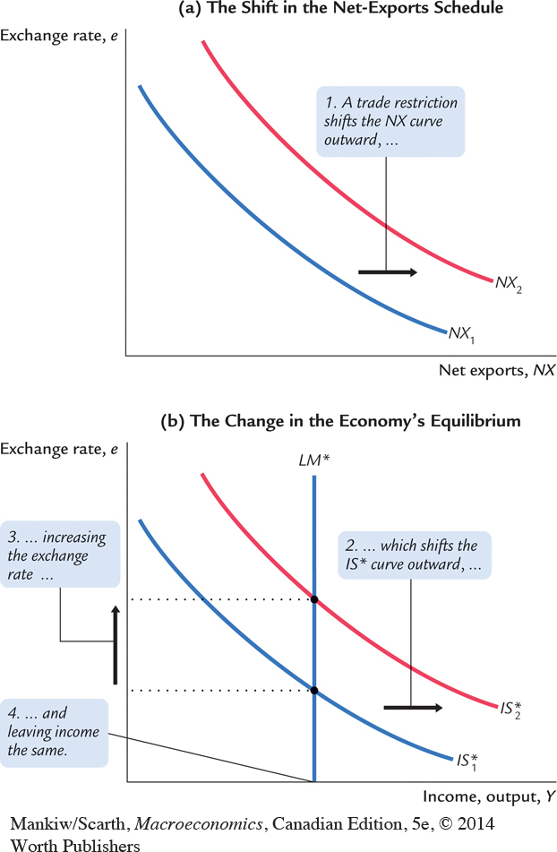
Because net exports equal exports minus imports, a reduction in imports means an increase in net exports. That is, the net-exports schedule shifts to the right, as in Figure 12-8. This shift in the net-exports schedule increases planned expenditure and thus moves the IS* curve to the right. Because the LM* curve is vertical, the trade restriction raises the exchange rate but does not affect income.
390
The economic forces behind this transition are similar to the case of expansionary fiscal policy. Because net exports are a component of GDP, the rightward shift in the net-exports schedule, other things equal, puts upward pressure on income Y; an increase in Y, in turn, increases money demand and puts upward pressure on the interest rate r. Foreign capital quickly responds by flowing into the domestic economy, pushing the interest rate back to the world interest rate r* and causing the domestic currency to appreciate in value. Finally, the appreciation of the currency makes domestic goods more expensive relative to foreign goods, which decreases net exports NX and returns income Y to its initial level.
Often a stated goal of policies to restrict trade is to alter the trade balance NX. Yet, as we first saw in Chapter 5, such policies do not necessarily have that effect. The same conclusion holds in the Mundell–Fleming model under floating exchange rates. Recall that
NX(e) = Y – C(Y – T ) – I(r *) – G.
Because a trade restriction does not affect income, consumption, investment, or government purchases, it does not affect the trade balance. Although the shift in the net-exports schedule tends to raise NX, the increase in the exchange rate reduces NX by the same amount. The overall effect is simply less trade. The domestic economy imports less than it did before the trade restriction, but it exports less as well.
World Interest-Rate Changes
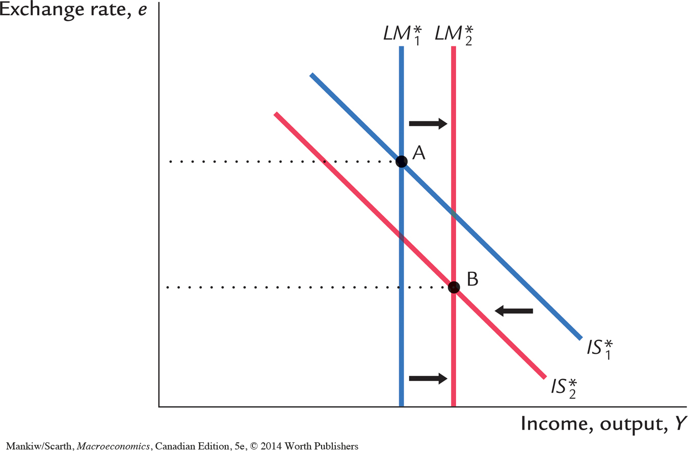
Consider an increase in the general level of world interest rates. In the Mundell–Fleming model, this means that Canadian interest rates must rise (as the law of one price operates in the world bond markets). But will this cause a rise or fall in the level of aggregate demand in Canada? Clearly, the higher borrowing cost will depress the investment spending component of aggregate demand, but can the exchange-rate change insulate aggregate demand from this depressing effect of higher interest rates? We now use the model to answer this question.
From Figure 12-5 we know that higher world interest rates cause LM* to shift to the right. Also, since higher interest rates depress firms’ investment spending on new plant and equipment, IS* shifts back to the left. These shifts are shown in Figure 12-9, where equilibrium moves from point A to point B. With funds initially leaving the country in pursuit of the high yields available in other parts of the world, the domestic currency depreciates, as shown in Figure 12-9. The model shows that this depreciation in the Canadian dollar must be of such a magnitude that aggregate demand rises. New exports are stimulated more than investment expenditure is reduced.2 Thus, one advantage of allowing a floating exchange rate is that we do not have to suffer a recession just because there are increases in either world tariffs or world interest rates.