12.3 The Small Open Economy Under Fixed Exchange Rates
391
We now turn to the second type of exchange-rate system: fixed exchange rates. Under a fixed exchange rate, the central bank announces a value for the exchange rate and stands ready to buy and sell the domestic currency to keep the exchange rate at its announced level. In the 1950s and 1960s, most of the world’s major economies operated within the Bretton Woods system—an international monetary system under which most governments agreed to fix exchange rates. The world abandoned this system in the early 1970s, and most exchange rates were allowed to float freely. Yet fixed exchange rates are not merely of historical interest. Some European countries have reinstated a system of fixed exchange rates among themselves (as a common currency, the euro, was introduced in 1999). More recently, China fixed the value of its currency against the U.S. dollar—a policy that, as we will see, was a source of some tension between the two countries. In this section we discuss how such a system works, and we examine the impact of economic policies on an economy with a fixed exchange rate. Later in the chapter we examine the pros and cons of fixed exchange rates.
How a Fixed-Exchange-Rate System Works
Under a system of fixed exchange rates, a central bank stands ready to buy or sell the domestic currency for foreign currencies at a predetermined price. Suppose, for example, that the Bank of Canada announced that it was going to fix the exchange rate at $0.90 (U.S.) per dollar. It would then stand ready to give $1 (Canadian) in exchange for $0.90 (U.S.) or to give $0.90 (U.S.) in exchange for $1 (Canadian). To carry out this policy, the Bank of Canada would need a reserve of Canadian dollars (which it can print) and a reserve of U.S. dollars (which it must have accumulated in past transactions).
392
A fixed exchange rate dedicates a country’s monetary policy to the single goal of keeping the exchange rate at the announced level. In other words, the essence of a fixed-exchange-rate system is the commitment of the central bank to allow the money supply to adjust to whatever level will ensure that the equilibrium exchange rate equals the announced exchange rate. Moreover, as long as the central bank stands ready to buy or sell foreign currency at the fixed exchange rate, the money supply adjusts automatically to the necessary level.
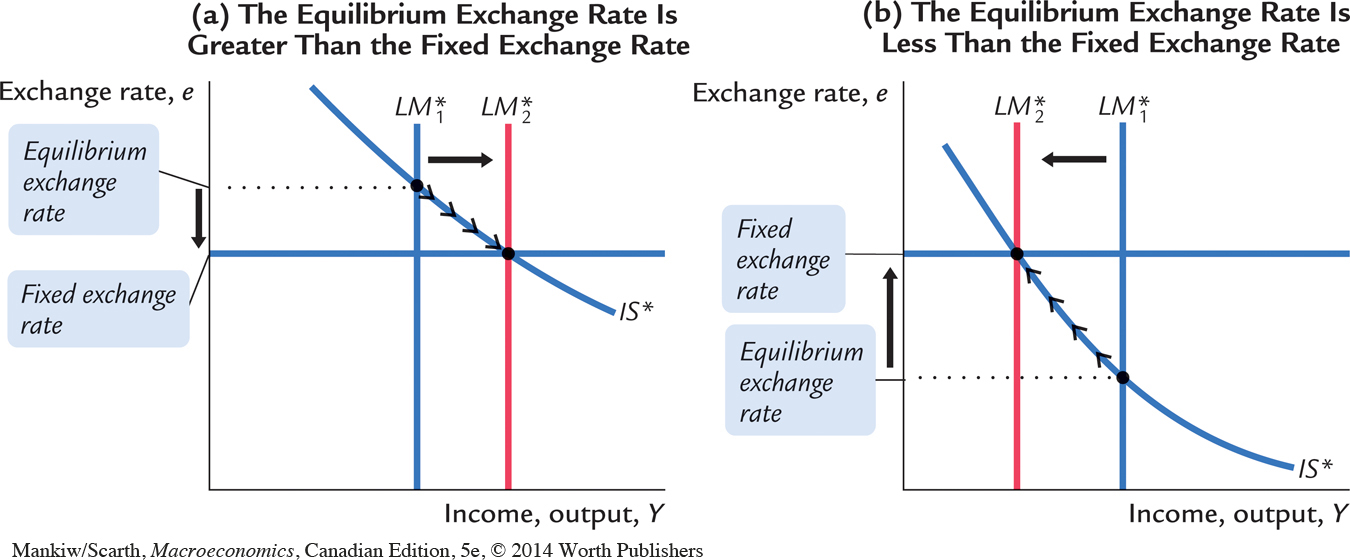
To see how fixing the exchange rate determines the money supply, consider the following example. Suppose that the Bank of Canada announces that it will fix the exchange rate at $0.90 (U.S.) per dollar, but, in the current equilibrium with the current money supply, the exchange rate is $0.95 (U.S.) per dollar. This situation is illustrated in panel (a) of Figure 12-10. Notice that there is a profit opportunity: an arbitrageur could buy $95 (U.S.) in the marketplace for $100 (Canadian), and then sell the U.S. dollars to the Bank of Canada for $105.55 ($95/$0.90); making a profit of $5.55. When the Bank of Canada buys these U.S. dollars from the arbitrageur, the Canadian dollars it pays for them automatically increase the domestic money supply. The rise in the money supply shifts the LM* curve to the right, lowering the equilibrium exchange rate. In this way, the money supply continues to rise until the equilibrium exchange rate falls to the announced level.
393
Conversely, suppose that the Bank of Canada announces that it will fix the exchange rate at $0.90 (U.S.) per dollar, when the equilibrium is $0.80 (U.S.) per dollar. Panel (b) of Figure 12-10 shows this situation. In this case, an arbitrageur could make a profit by buying $90 (U.S.) from the Bank of Canada for $100 and then selling the U.S. dollars in the marketplace for $112.50 Canadian ($90/$0.80). When the Bank of Canada sells these U.S. dollars, the Canadian dollars it receives are no longer circulating among private transactors, so this policy automatically reduces the money supply. The fall in the money supply shifts the LM* curve to the left, raising the equilibrium exchange rate. The money supply continues to fall until the equilibrium exchange rate rises to the announced level.
These examples make clear that fixing the exchange rate requires a commitment on the part of the Bank of Canada to either buy or sell whatever amount of foreign exchange is demanded by private participants in foreign-currency markets. Fixing a Canadian dollar price below the free-market equilibrium can be done indefinitely, because all the Bank of Canada needs is an unlimited supply of Canadian dollars (which it can print). Nevertheless, this policy is limited by the willingness of Canadians to tolerate the inflation that eventually accompanies rapid growth in the domestic money supply.
Fixing the Canadian dollar at a price above the free-market equilibrium, on the other hand, cannot be done indefinitely. This follows from the basic fact that the Bank of Canada cannot print foreign exchange. Private traders know this, and they can easily determine how rapidly the Bank of Canada’s reserves of foreign exhange are running out. Canada’s balance of payments data record precisely this—the amount by which the country’s foreign exchange reserves have been depleted each period. Armed with this information, private traders can readily guess when the Bank of Canada will have to give up fixing the exchange rate at such a high value. It is in this situation that we hear about a “speculative run against the currency” in the media. Once private traders see that a country’s currency is about to fall in value, they sell off that currency to avoid the almost certain capital loss. This very action hastens the exchange-rate change and verifies the speculator’s expectations.
It is important to understand that this exchange-rate system fixes the nominal exchange rate. Whether it also fixes the real exchange rate depends on the time horizon under consideration. If prices are flexible, as they are in the long run, then the real exchange rate can change even while the nominal exchange rate is fixed. Therefore, in the long run described in Chapter 5, a policy to fix the nominal exchange rate would not influence any real variable, including the real exchange rate. A fixed nominal exchange rate would influence only the money supply and the price level. Yet in the short run described by the Mundell–Fleming model, prices are fixed, so a fixed nominal exchange rate implies a fixed real exchange rate as well.
394
CASE STUDY
The International Gold Standard
During the late nineteenth and early twentieth centuries, most of the world’s major economies operated under a gold standard. Each country maintained a reserve of gold and agreed to exchange one unit of its currency for a specified amount of gold. Through the gold standard, the world’s economies maintained a system of fixed exchange rates.
To see how an international gold standard fixes exchange rates, suppose that the U.S. Treasury stands ready to buy or sell 1 ounce of gold for $100, and the Bank of England stands ready to buy or sell 1 ounce of gold for 100 pounds. Together, these policies fix the rate of exchange between dollars and pounds: $1 must trade for 1 pound. Otherwise, the law of one price would be violated, and it would be profitable to buy gold in one country and sell it in the other.
Suppose, for example, that the market exchange rate were 2 pounds per dollar. In this case, an arbitrageur could buy 200 pounds for $100, use the pounds to buy 2 ounces of gold from the Bank of England, bring the gold to the United States, and sell it to the Treasury for $200—making a $100 profit. Moreover, by bringing the gold to the United States from England, the arbitrageur would increase the money supply in the United States and decrease the money supply in England.
Thus, during the era of the gold standard, the international transport of gold by arbitrageurs was an automatic mechanism adjusting the money supply and stabilizing exchange rates. This system did not completely fix exchange rates, because shipping gold across the Atlantic was costly. Yet the international gold standard did keep the exchange rate within a range dictated by transportation costs. It thereby prevented large and persistent movements in exchange rates.3 
Fiscal Policy
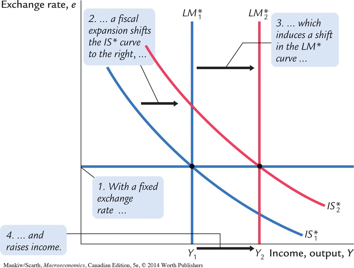
Let’s now examine how economic policies affect a small open economy with a fixed exchange rate. Suppose that the government stimulates domestic spending by increasing government purchases or by cutting taxes. This policy shifts the IS* curve to the right, as in Figure 12-11, putting upward pressure on the market exchange rate. But because the central bank stands ready to trade foreign and domestic currency at the fixed exchange rate, arbitrageurs quickly respond to the rising exchange rate by selling foreign currency to the central bank, leading to an automatic monetary expansion. The rise in the money supply shifts the LM* curve to the right. Thus, in contrast to the situation under floating exchange rates, a fiscal expansion under fixed exchange rates raises aggregate income.
Monetary Policy
395
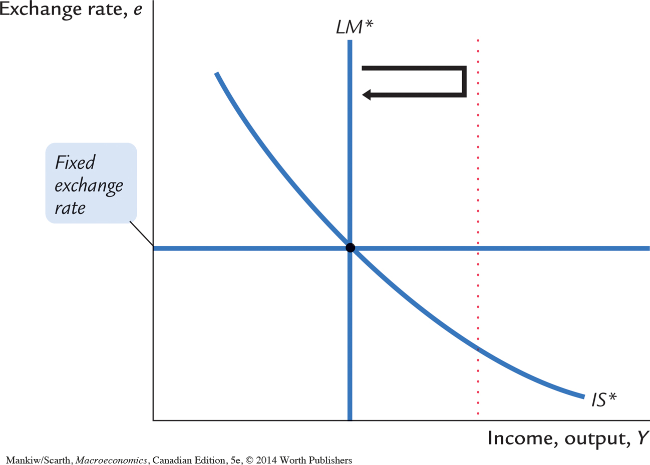
Imagine that a central bank operating with a fixed exchange rate were to try to increase the money supply—for example, by buying bonds from the public. What would happen? The initial impact of this policy is to shift the LM* curve to the right, lowering the exchange rate, as in Figure 12-12. But, because the central bank is committed to trading foreign and domestic currency at a fixed exchange rate, arbitrageurs quickly respond to the falling exchange rate by selling the domestic currency to the central bank, causing the money supply and the LM* curve to return to their initial positions. Hence, monetary policy as usually conducted is ineffectual under a fixed exchange rate. By agreeing to fix the exchange rate, the central bank gives up its control over the money supply.
396
A country with a fixed exchange rate can, however, conduct a type of monetary policy: it can decide to change the level at which the exchange rate is fixed. A reduction in the official value of the currency is called a devaluation, and an increase in its official value is called a revaluation. In the Mundell–Fleming model, a devaluation shifts the LM* curve to the right; it acts like an increase in the money supply under a floating exchange rate. A devaluation thus expands net exports and raises aggregate income. Conversely, a revaluation shifts the LM* curve to the left, reduces net exports, and lowers aggregate income.
CASE STUDY
Devaluation and the Recovery From the Great Depression
The Great Depression of the 1930s was a global problem. Although events in the United States may have precipitated the downturn for many other Western countries like Canada, all of the world’s major economies experienced huge declines in production and employment. Yet not all governments responded to this calamity in the same way.
One key difference among governments was how committed they were to the fixed exchange rate set by the international gold standard. Some countries, such as France, Germany, Italy, and the Netherlands, maintained the old rate of exchange between gold and currency. Other countries, such as Denmark, Finland, Norway, Sweden, and the United Kingdom, reduced the amount of gold they would pay for each unit of currency by about 50 percent. By reducing the gold content of their currencies, these governments devalued their currencies relative to those of other countries.
The subsequent experience of these two groups of countries conforms to the prediction of the Mundell–Fleming model. Those countries that pursued a policy of devaluation recovered quickly from the Depression. The lower value of the currency stimulated exports and expanded production. By contrast, those countries that maintained the old exchange rate suffered longer with a depressed level of economic activity.4
Trade Policy
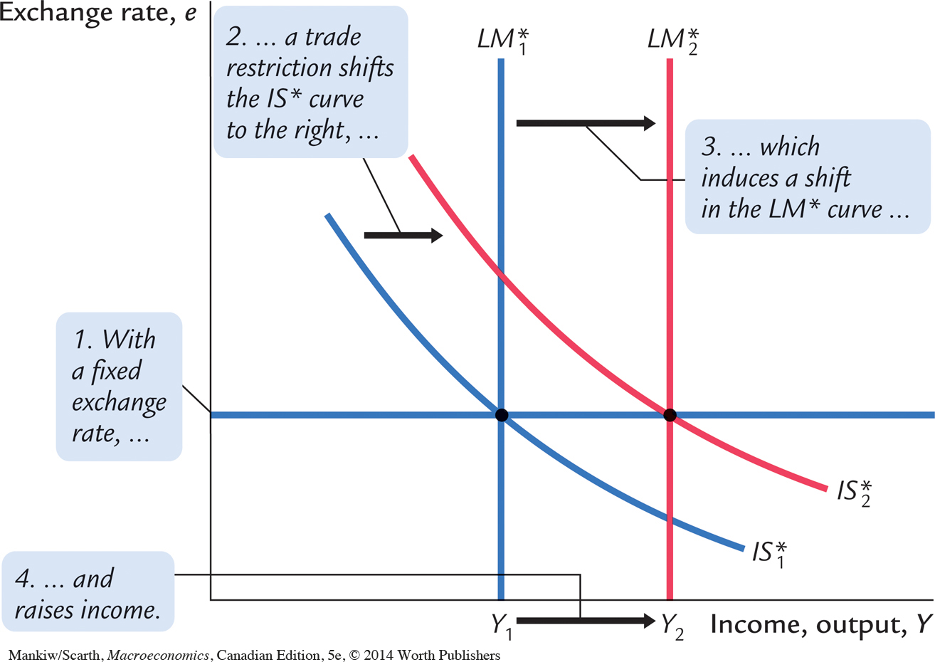
Suppose that the government reduces imports by imposing an import quota or a tariff. This policy shifts the net-exports schedule to the right and thus shifts the IS* curve to the right, as in Figure 12-13. The shift in the IS* curve tends to raise the exchange rate. To keep the exchange rate at the fixed level, the money supply must rise, shifting the LM* curve to the right.
397
The result of a trade restriction under a fixed exchange rate is very different from that under a floating exchange rate. In both cases, a trade restriction shifts the net-exports schedule to the right, but only under a fixed exchange rate does a trade restriction increase net exports NX. The reason is that a trade restriction under a fixed exchange rate induces monetary expansion rather than an appreciation of the exchange rate. The monetary expansion, in turn, raises aggregate income. Recall the accounting identity
NX = S – I.
When income rises, saving also rises, and this implies an increase in net exports.
This analysis can be used to consider tariffs levied by foreigners as well. In that case, our net exports are reduced so the shifts in IS* and LM* are to the left, instead of to the right (as they are in Figure 12-13). In contrast to the floating-exchange-rate case, then, Canada must suffer a recession following the imposition of foreign trade restrictions, if the exchange rate is fixed.
Similarly, if we have a fixed exchange rate, we must suffer a recession if world commodity prices change—as they did in the 1990s during the Asian crisis—to reduce Canadian net exports. At the time of the Asian crisis, Canada had a floating exchange rate. While the dip in the Canadian dollar (down to $0.63 (U.S.) in mid-1998) caused concern, it did provide Canada some insulation from this major event. While our exports of primary commodities suffered during the Asian crisis, at least our manufacturing exports were stimulated by the lower domestic currency. Many analysts concluded that it was fortunate that Canada had not opted for a fixed exchange rate at this time.
World Interest-Rate Changes
398
The analysis of foreign interest-rate increases under fixed exchange rates is similar to that for trade restrictions imposed by other countries. Higher interest rates lower investment spending by firms, so IS* shifts to the left for this reason, rather than because of a reduction in net exports. However, whatever causes the IS* curve to shift is insignificant; LM* must still shift to the left to keep the exchange rate fixed. (Just picture Figure 12-13 running in reverse.) Thus, Canada must suffer a recession following an increase in world interest rates if the exchange rate is fixed.
This same analysis applies to small open economies in Europe that have maintained fixed exchange rates with one another. In the early 1990s, German reunification meant a big increase in government spending to improve conditions in the former East Germany. Given the commitment to low inflation on the part of the German central bank, this spending led to higher German interest rates. Our model shows that the only way that the other European countries could avoid a recession—that would otherwise accompany this increase in interest rates caused by the changes happening in Germany—was to shift away from fixed exchange rates. This is exactly what happened in 1992.
Policy in the Mundell–Fleming Model: A Summary
The Mundell–Fleming model shows that the effect of almost any economic policy on a small open economy depends on whether the exchange rate is floating or fixed. Table 12-1 summarizes our analysis of the short-run effects of fiscal, monetary, and trade policies, and world interest rate changes, on income, the exchange rate, and the trade balance. What is most striking is that all of the results are different under floating and fixed exchange rates.
| EXCHANGE-RATE REGIME | ||||||
| FLOATING | FIXED | |||||
| IMPACT ON: | ||||||
| Policy/World Event | Y | e | NX | Y | e | NX |
| Fiscal expansion | 0 | ↑ | ↓ | ↑ | 0 | 0 |
| Monetary expansion | ↑ | ↓ | ↑ | 0 | 0 | 0 |
| Import restriction | 0 | ↑ | 0 | ↑ | 0 | ↑ |
| Export restriction | 0 | ↓ | 0 | ↓ | 0 | ↓ |
| Higher interest rates | ↑ | ↓ | ↑ | ↓ | 0 | 0 |
|
Note: This table shows the direction of impact of various economic policies on income Y, the exchange rate e, and the trade balance NX. A “↑” indicates that the variable increases; a “↓” indicates that it decreases; a “0” indicates no effect. Remember that the exchange rate is defined as the amount of foreign currency per unit of domestic currency (for example, $0.90 (U.S.)/Canadian dollar). |
||||||
|---|---|---|---|---|---|---|
399
To be more specific, the Mundell–Fleming model shows that the power of monetary and fiscal policy to influence aggregate income depends on the exchange-rate regime. Under floating exchange rates, only monetary policy can affect income. The usual expansionary impact of fiscal policy is offset by a rise in the value of the currency and a decrease in net exports. Under fixed exchange rates, only fiscal policy can affect income. The normal potency of monetary policy is lost because the money supply is dedicated to maintaining the exchange rate at the announced level.
CASE STUDY
Regional Tensions Within Canada
The Mundell–Fleming model can be used to help explain why regional tensions increased in Canada during the late 1980s. At that time, the Ontario government was running an expansionary fiscal policy. We now know that the overall impact of such a policy (throughout the country) is that it has no effect on aggregate demand. Instead it creates a higher Canadian dollar, which forces net exports to be reduced by the same amount as government spending is increased. But consider the distribution of these two effects within the country.
The increase in the government spending component of aggregate demand is concentrated entirely within Ontario, whereas the crowding out of preexisting net export demand is felt in all provinces. The result is that demand in Ontario is increased, while that in the rest of the country is decreased. The two effects add up to zero as far as overall demand in the entire country is concerned. Thus, fiscal policy does work under floating exchange rates after all, but only from one province’s point of view. Ontario can reduce its unemployment problem, but only by worsening the same problem for the other regions!