417

APPENDIX

Extensions to the Mundell–Fleming Model

One of the most important properties of the Mundell–Fleming model is the insulation a flexible exchange rate provides in the face of demand shocks. As we discovered in the main text of this chapter, a reduction in demand leads to a lower domestic currency, which stimulates net exports. With new jobs created in the export- and import-competing sectors—to replace those lost due to the initial drop in demand—a floating exchange rate provides the economy with an automatic stabilizer. Why is it that a number of countries are prepared to give up this automatic stabilizer? Perhaps policymakers in these countries feel that the Mundell–Fleming model is too simplified. We explore this question in this appendix by examining whether the property of insulation from demand shocks remains as the model is extended.

Three extensions are considered. First, since the exchange rate is an important determinant of the domestic price of imports, we allow the exchange rate to have a direct effect on the consumer price index (CPI). Second, we allow domestic prices and wages to be endogenous. Third, we consider endogenous exchange-rate expectations.

Households buy both domestically produced goods and imports. If we use P^d, P^f, and λ to denote the price of domestically produced goods, the price of foreign goods (denominated in foreign currency), and the proportion of each household budget that is devoted to domestically produced goods, the consumer price index can be written as

P = λP^d+ (1 – λ)P^f/e.

(P^f/e) is the price of imports in domestic currency units.

With respect to prices, two simplifications are involved in the Mundell–Fleming model. First, fixed prices—both at home and abroad—are assumed. This simplification involves setting P^d = P^f = 1. Second, the price of domestically produced goods, P^d, and the overall consumer price index, P, are assumed to be the same thing. By focusing on the formal definition of the CPI, we can see that this second simplification is inappropriate. Even with P^d = P^f = 1, the consumer price index is not constant. Indeed, it must change whenever the exchange rate does:

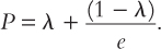
P = λ + (1 – λ)/e.

418

The revised model becomes

Y = C(Y – T) I (r*) + G + NX(e),

M/P = L (Y, r*),

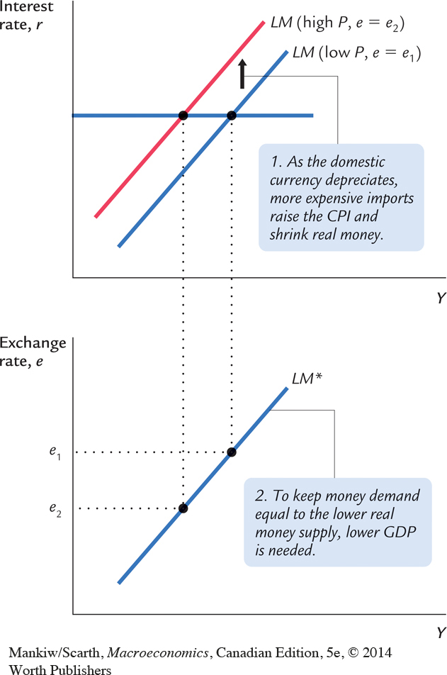
Compared to the basic Mundell–Fleming model, this extension involves the exchange rate affecting the money market. (Once the third equation is used to replace P in the LM* equation, we can see that e becomes an important part of that relationship.) Given this complication, we must re-derive the LM* locus. This is accomplished in Figure 12-18. There we see that, because a lower domestic currency makes imports more expensive, the CPI is higher when e is lower. As a result, the real money supply is smaller when the domestic currency falls in value, and the LM curve in panel (a) shifts to the left. The positive slope of the LM* locus in panel (b) summarizes this outcome.

419

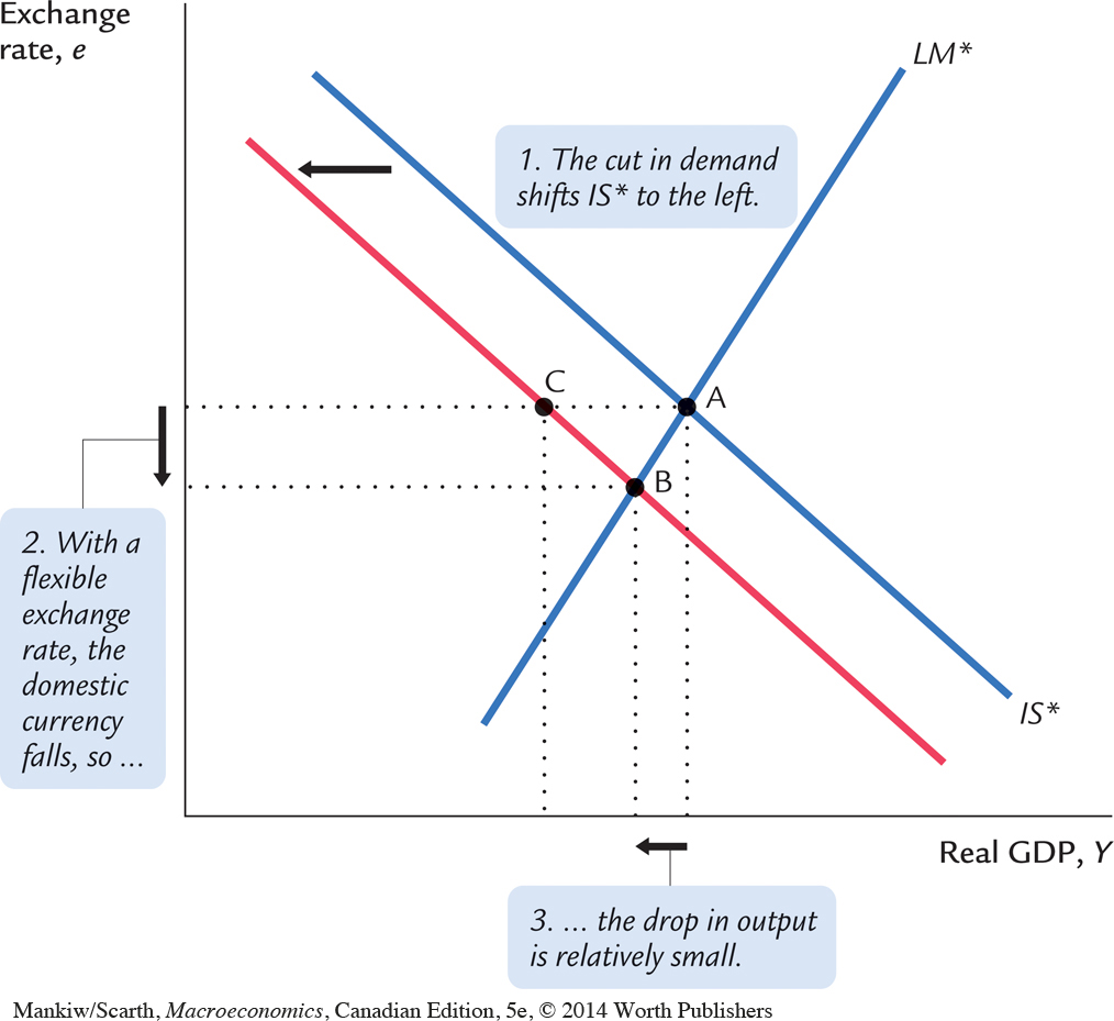
We are now in a position to reassess the insulation property. A drop in demand—perhaps caused by lower government spending—shifts IS* to the left as usual. The revised result is shown in Figure 12-19. With a floating exchange rate, the economy moves from A to B; with a fixed exchange rate, the central bank must move LM* to the left and the economy moves from A to C. (Only the final outcome, not the shift in LM*, is shown in Figure 12-19.) Since output falls in both scenarios, a floating exchange rate no longer provides complete insulation from demand shocks. Nevertheless, since the fall in output is less with a floating rate, some insulation still remains. It is important to note a second difference between the fixed- and flexible-exchange-rate cases. The CPI is not affected under fixed rates, while the CPI must rise under floating rates. This is one reason why some countries have opted for fixed exchange rates. A floating rate provides some (but reduced) insulation for real output, but that insulation is “purchased” at the expense of having to accept an increase in the general cost of living. In short, under floating rates, a decrease in spending is like an oil price increase—it is stagflationary.

420

Let us continue extending the Mundell–Fleming model by letting P^d become an endogenous variable. Just to illustrate how this extension can affect the model’s properties, we focus on one special case. We assume that the price of domestically produced goods adjusts one-for-one with changes in wages,

and we assume that wages adjust one-for-one with changes in the overall cost of living,

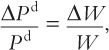
Together, these relationships imply ΔP^d/P^d = ΔP/P. When this condition is substituted into the percentage-change version of the consumer price index,

we have

ΔP^d/P^d = ΔP/P = (ΔP^f/P^f – Δe/e)

which implies that the real exchange rate, eP^d/P^f, is constant.

The revised IS relationship is

Since the real exchange rate is fixed, the IS* locus that follows from this relationship is vertical, and the effect of a drop in government spending is shown in Figure 12-20. The economy moves from point A to B under flexible exchange rates, and from A to C with a fixed rate. Since the effect on real output is the same, the insulation feature of a floating exchange rate is lost completely. While the direct effect of a falling domestic currency remains favourable (it stimulates demand for domestically produced goods), the model now contains an indirect effect that is unfavourable (the falling domestic currency raises the general cost of living, and therefore wages). Higher domestic costs make the economy less competitive. In this specific model, the direct and indirect effects of the falling dollar just cancel.

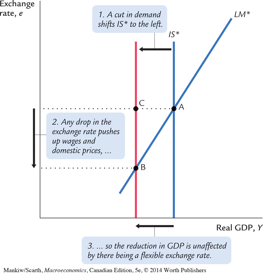
This version of the model gives even more support for those who choose a fixed exchange rate. In this case, a fixed exchange rate does not involve giving up any built-in stability, and we avoid the increase in the cost of living (which accompanies a drop in spending only in the flexible-exchange-rate case).

The choice with respect to the exchange-rate regime seems to depend on whether a country’s labour-market institutions lead to sticky nominal wages or sticky real wages in the short run. In many European countries there is a synchronized annual adjustment in most nominal wage rates (and this adjustment reflects the previous year’s increase in the CPI). As a result, the present version of our model seems particularly suited to European countries, and their adoption of a common currency is therefore supported by the analysis. In North America, on the other hand, many workers have wage contracts that stipulate the nominal wage for a considerable time into the future. As a result, most economists are more comfortable assuming sticky nominal wages, not sticky real wages, for Canada and the United States. This presumption makes the earlier version of the Mundell–Fleming model more appropriate for Canada; and this analysis supports our decision to reject currency union with the United States (fixed exchange rates).

421

To keep things relatively straightforward in this discussion of exchange-rate expectations, let us revert to the P^d= P^f = 1 simplification. In the main text of this chapter we noted that perfect capital mobility forces the domestic interest rate to equal the foreign rate plus the risk premium:

r = r* + θ.

Thus far, we have limited our attention to exogenous changes in θ. The purpose of this part of the appendix is to consider θ as an endogenous variable.

422

We know that θ must rise whenever asset holders expect the domestic currency to fall. Since our currency does fall (under flexible exchange rates) when there is a drop in government spending, let us now add this expectation effect to our analysis of fiscal retrenchment.

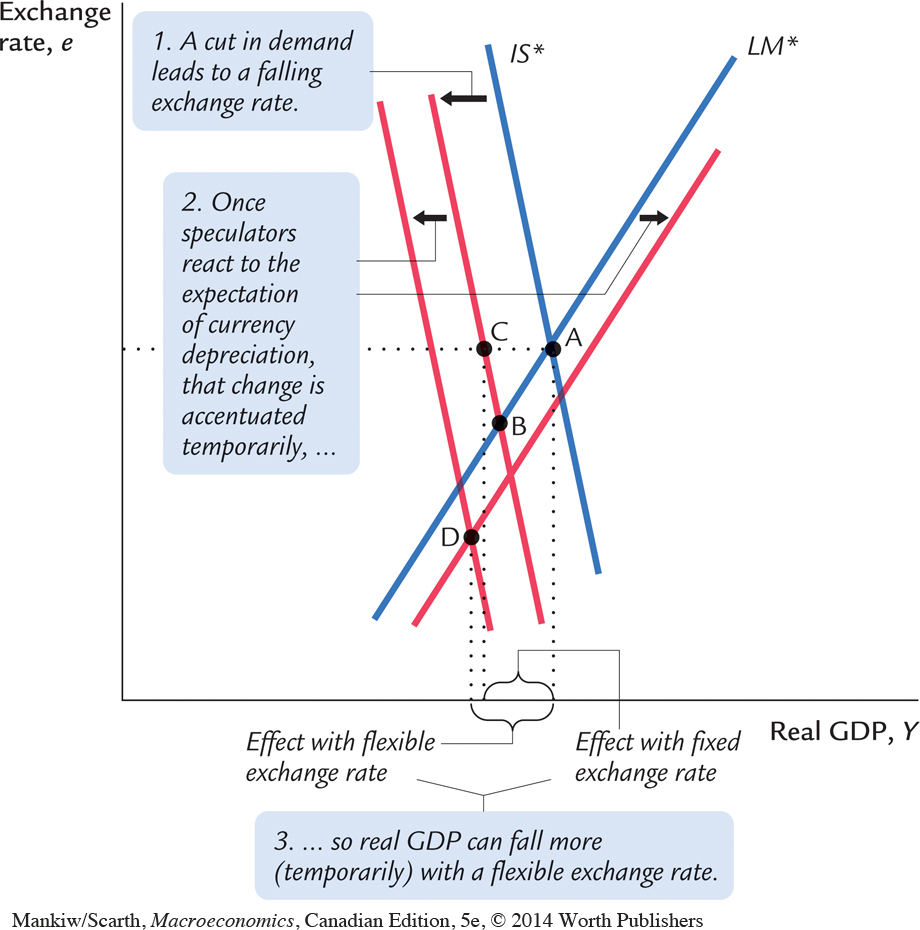
We saw the outcome of a reduction in G in Figure 12-19—when there was no risk-premium effect. At least as far as avoiding part of an undesirable drop in real output is concerned, a floating exchange rate is appealing; it allows the economy to move to point B, not point C. But since well-informed individuals understand that this drop in the domestic currency will occur, they will adjust their expectations, and θ will rise accordingly. In the main text of this chapter, we learned that such a rise in θ must shift the IS* locus to the left (since higher interest rates lower investment spending) and shift the LM* locus to the right (since higher interest rates reduce money demand). Once these additional shifts are added (in Figure 12-21), we see that the more complete comparison of the outcomes under alternative exchange-rate regimes is a move from A to C with a fixed exchange rate, and a move from A to D under flexible rates. As is shown in the figure, point D may be just as far to the left as point C. If so, a floating rate does not operate as a built-in stabilizer with respect to real output outcomes.

423

Of course, these additional shifts in the IS* and LM* loci are only temporary, since once the exchange rate stops changing, θ will return to zero. This consideration leads many policymakers to opt for a floating exchange rate but to intervene in an ongoing fashion to smooth out the short-run variations in the exchange rate. (This is called managed floating.) But it is easy to see that such an attempt to smooth the exchange rate may backfire. To appreciate this fact, consider rewriting the interest arbitrage condition, r = r* + θ.

Let θ be represented by the expected depreciation in the domestic currency, which we can denote as – (e – e^exp), where e^exp stands for the expected exchange rate. Also, let the interest-rate deviation (r* – r) be represented by the random variable v. The interest-arbitrage relationship then becomes:

e_t = e_t^exp + v_t.

The t subscripts denote the current time period. In forming expectations about the exchange rate, it is reasonable to assume that individuals will put some weight on where they expect the exchange rate to be going (its full equilibrium value, e*) and some weight on where the exchange rate has been (its value in the previous time period, e_t−1). Letting those weights be (1 – γ) and γ, expectation formation is given by

e_t^exp = (1 – γ)e* + γe_t-1.

Substituting this expression into the interest arbitrage condition, we have

e_t = (1 – γ)e* + γe_t–1 + v_t.

Simple examination of this relationship indicates that exchange-rate volatility is smallest when γ is zero. Suppose that the random disturbance term, v_t, is nonzero for just one period. If γ is zero, the exchange rate will be affected for just that one period. But if γ is positive, the effect of that one disturbance will last for many periods. For example, if γ is one-half, the exchange rate will still be affected by one-half of the original amount one period later, and by one-quarter of the original amount two periods later, and so on.

So low volatility in the exchange rate requires a low value of γ. But if individuals know that the central bank is smoothing the exchange rate, they have every reason to put a large weight on the previous period’s value when forming expectations. Thus, the more the central bank tries to smooth the exchange rate, the more rational it is for individuals to choose a high value for γ, and the more volatile is the exchange rate after all.

This conclusion is an example of the Lucas critique (discussed in Chapter 15). Exchange-rate smoothing makes sense if the direct effect of policy on expectation formation is ignored, but not otherwise. Partly because of this ambiguity, many central banks have opted for stabilizing the rate of inflation, not the exchange rate.

In a world of capital mobility, with speculators constantly on the lookout for fixed-exchange-rate promises to “test,” the most credible form of fixed exchange rates is currency union. In Canada’s case, this means eliminating the Canadian dollar and using the U.S. dollar as our currency. This choice has been hotly debated in the media.

424

The main advantage of currency union is the possibility that a lower risk premium could bring lower interest rates and a higher capital/labour ratio. However, with the U.S. Fed pursuing roughly the same inflation rate as the Bank of Canada, there is little basis for choice on this criterion. Without negotiation, however, Canadians would relinquish seigniorage revenue (a small consideration) and lender-of-last-resort facilities for financial crises (a significant consideration, as the events of 2008 have reminded us) by choosing currency union. The final issue concerns whether a separate currency imparts built-in stability to the economy. The basic answer to this question, which follows from our series of extensions to the Mundell–Fleming model, is that a floating rate does act as a buffer. This shock-absorber property is often exaggerated to a significant degree, but as long as Canada approximates what Mundell has called an “optimum currency area,” it is likely that some of this property of flexible exchange rates will remain.

To appreciate what is meant by an optimum currency area, it is instructive to think of North America divided in two ways—first between north and south, and second between west and east. First, assume that the north produces wheat and the south produces cars. A shift in tastes (higher demand for cars and lower demand for wheat) results in inflation in the south and unemployment in the north. If there is a separate currency for the north and a floating exchange rate, a depreciating northern currency can reduce both the inflation and unemployment problems. Now assume that the west produces wheat and the east produces cars. The same shift in tastes causes inflation in the east and unemployment in the west. As before, if there is a separate currency for the west, a flexible exchange rate is a substitute for factor mobility, so it can decrease the costs of adjusting to the change in tastes.

In the first scenario, north and south are the areas for which it would be helpful to have separate currencies; in the second scenario, it is the east and west that represent optimum currency areas. The problem in North America is that—over time—the second scenario is becoming the more relevant one, while currencies are still based on our national border (north versus south). The greater this mismatch is, the less sense it makes (on short-run macroeconomic stability grounds) to maintain a separate Canadian currency. As a result, we can expect the debate on Canada’s exchange-rate policy to continue. It is interesting to note that, as Mundell has contributed to the development of open-economy macroeconomics following his original model, he has argued—increasingly over time—for a return to fixed exchange rates.