13.1 The Basic Theory of Aggregate Supply
426
When students in physics classes study balls rolling down inclined planes, they often begin by assuming away the existence of friction. This assumption makes the problem simpler and is useful in many circumstances, but no good engineer would ever take this assumption as a literal description of how the world works. Similarly, this book began with classical macroeconomic theory, but it would be a mistake to assume that this model is true in all circumstances. Our job now is to look more deeply into the “frictions” of macroeconomics.
We do this by examining two prominent models of aggregate supply. In both models, some market imperfection (that is, some type of friction) causes the output of the economy to deviate from its natural level. As a result, the short-run aggregate supply curve is upward sloping, rather than vertical, and shifts in the aggregate demand curve cause output to fluctuate. These temporary deviations of output from its natural level represent the booms and busts of the business cycle.
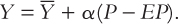
Each of the two models takes us down a different theoretical route, but each route ends up in the same place. That final destination is a short-run aggregate supply equation of the form

where Y is output,  is the natural level of output, P is the price level, and EP is the expected price level. This equation states that output deviates from its natural level when the price level deviates from the expected price level. The parameter a indicates how much output responds to unexpected changes in the price level; 1/α is the slope of the aggregate supply curve.
Each of the models tells a different story about what lies behind this short-run aggregate supply equation. In other words, each model highlights a particular reason why unexpected movements in the price level are associated with fluctuations in aggregate output.
The Sticky-Price Model
427
The most widely accepted explanation for the upward-sloping short-run aggregate supply curve is called the sticky-price model. This model emphasizes that firms do not instantly adjust the prices they charge in response to changes in demand. Sometimes prices are set by long-term contracts between firms and customers. Even without formal agreements, firms may hold prices steady to avoid annoying their regular customers with frequent price changes. Some prices are sticky because of the way markets are structured: once a firm has printed and distributed its catalogue or price list, it is costly to alter prices. And sometimes sticky prices can be a reflection of sticky wages: firms base their prices on the costs of production, and wages may depend on social norms and notions of fairness that evolve only slowly over time.
There are various ways to formalize the idea of sticky prices to show how they can help explain an upward-sloping aggregate supply curve. Here we examine an especially simple model. We first consider the pricing decisions of individual firms and then add together the decisions of many firms to explain the behaviour of the economy as a whole. To fully understand the model, we have to depart from the assumption of perfect competition, which we have used since Chapter 3. Perfectly competitive firms are price takers rather than price setters. If we want to consider how firms set prices, it is natural to assume that these firms have at least some monopolistic control over the prices they charge.
Consider the pricing decision facing a typical firm. The firm’s desired price p depends on two macroeconomic variables:
The overall level of prices P. A higher price level implies that the firm’s costs are higher. Hence, the higher the overall price level, the more the firm would like to charge for its product.
The level of aggregate income Y. A higher level of income raises the demand for the firm’s product. Because marginal cost increases at higher levels of production, the greater the demand, the higher the firm’s desired price.
We write the firm’s desired price as
This equation says that the desired price p depends on the overall level of prices P and on the level of aggregate output relative to the natural level Y –
. The parameter a (which is greater than zero) measures how much the firm’s desired price responds to the level of aggregate output.1
Now assume that there are two types of firms. Some have flexible prices: they always set their prices according to this equation. Others have sticky prices: they announce their prices in advance based on what they expect economic conditions to be. Firms with sticky prices set prices according to
428
where, as before, an “E” represents the expected value of a variable. For simplicity, assume that these firms expect output to be at its natural rate, so that the last term, a(EY – E
), is zero. Then these firms set the price
p = EP.
That is, firms with sticky prices set their prices based on what they expect other firms to charge.
We can use the pricing rules of the two groups of firms to derive the aggregate supply equation. To do this, we find the overall price level in the economy, which is the weighted average of the prices set by the two groups. If s is the fraction of firms with sticky prices and 1 – s the fraction with flexible prices, then the overall price level is

The first term is the price of the sticky-price firms weighted by their fraction in the economy, and the second term is the price of the flexible-price firms weighted by their fraction. Now subtract (1 – s)P from both sides of this equation to obtain

Divide both sides by s to solve for the overall price level:

The two terms in this equation are explained as follows:
When firms expect a high price level, they expect high costs. Those firms that fix prices in advance set their prices high. These high prices cause the other firms to set high prices also. Hence, a high expected price level EP leads to a high actual price level P.
When output is high, the demand for goods is high. Those firms with flexible prices set their prices high, which leads to a high price level. The effect of output on the price level depends on the proportion of firms with flexible prices.
Hence, the overall price level depends on the expected price level and on the level of output.
Algebraic rearrangement puts this aggregate pricing equation into a more familiar form:
Where α = s/[(1 – s)a]. Like the other models, the sticky-price model says that the deviation of output from the natural level is positively associated with the deviation of the price level from the expected price level.2
An Alternative Theory: The Imperfect-Information Model
429
Another explanation for the upward slope of the short-run aggregate supply curve is called the imperfect-information model. Unlike the previous model, this one assumes that markets clear—that is, all prices are free to adjust to balance supply and demand. In this model, the short-run and long-run aggregate supply curves differ because of temporary misperceptions about prices.
The imperfect-information model assumes that each supplier in the economy produces a single good and consumes many goods. Because the number of goods is so large, suppliers cannot observe all prices at all times. They monitor closely the prices of what they produce but less closely the prices of all the goods they consume. Because of imperfect information, they sometimes confuse changes in the overall level of prices with changes in relative prices. This confusion influences decisions about how much to supply, and it leads to a short-run relationship between the price level and output.
Consider the decision facing a single supplier—a wheat farmer, for instance. Because the farmer earns income from selling wheat and uses this income to buy goods and services, the amount of wheat she chooses to produce depends on the price of wheat relative to the prices of other goods and services in the economy. If the relative price of wheat is high, the farmer is motivated to work hard and produce more wheat, because the reward is great. If the relative price of wheat is low, she prefers to enjoy more leisure and produce less wheat.
Unfortunately, when the farmer makes her production decision, she does not know the relative price of wheat. As a wheat producer, she monitors the wheat market closely and always knows the nominal price of wheat. But she does not know the prices of all the other goods in the economy. She must, therefore, estimate the relative price of wheat using the nominal price of wheat and her expectation of the overall price level.
Consider how the farmer responds if all prices in the economy, including the price of wheat, increase. One possibility is that she expected this change in prices. When she observes an increase in the price of wheat, her estimate of its relative price is unchanged. She does not work any harder.
The other possibility is that the farmer did not expect the price level to increase (or to increase by this much). When she observes the increase in the price of wheat, she is not sure whether other prices have risen (in which case wheat’s relative price is unchanged) or whether only the price of wheat has risen (in which case its relative price is higher). The rational inference is that some of each has happened. In other words, the farmer infers from the increase in the nominal price of wheat that its relative price has risen somewhat. She works harder and produces more.
Our wheat farmer is not unique. Her decisions are similar to those of her neighbours, who produce broccoli, cauliflower, dill, endive, and zucchini. When the price level rises unexpectedly, all suppliers in the economy observe increases in the prices of the goods they produce. They all infer, rationally but mistakenly, that the relative prices of the goods they produce have risen. They work harder and produce more.
430
To sum up, the imperfect-information model says that when prices exceed expected prices, suppliers raise their output. The model implies an aggregate supply curve that is now familiar:
Output deviates from the natural level when the price level deviates from the expected price level.
The imperfect-information story described above is the version developed originally by Nobel Prize–winning economist Robert Lucas in the 1970s. Recent work on imperfect-information models of aggregate supply has taken a somewhat different approach. Rather than emphasizing confusion about relative prices and the absolute price level, as Lucas did, this new work stresses the limited ability of individuals to incorporate information about the economy into their decisions. In this case, the friction that causes the short-run aggregate supply curve to be upward sloping is not the limited availability of information; it is, instead, the limited ability of people to absorb and process information that is widely available. This information-processing constraint causes price-setters to respond slowly to macroeconomic news. The resulting equation for short-run aggregate supply is similar to those from the two models we have seen, even though the microeconomic foundations are somewhat different.3
CASE STUDY
International Differences in the Aggregate Supply Curve
Although all countries experience economic fluctuations, these fluctuations are not exactly the same everywhere. International differences are intriguing puzzles in themselves, and they often provide a way to test alternative economic theories. Examining international differences has been especially fruitful in research on aggregate supply.
431
When Robert Lucas proposed the imperfect-information model, he derived a surprising interaction between aggregate demand and aggregate supply: according to his model, the slope of the aggregate supply curve should depend on the variability of aggregate demand. In countries where aggregate demand fluctuates widely, the aggregate price level fluctuates widely as well. Because most movements in prices in these countries do not represent movements in relative prices, suppliers should have learned not to respond much to unexpected changes in the price level. Therefore, the aggregate supply curve should be relatively steep (that is, a will be small). Conversely, in countries where aggregate demand is relatively stable, suppliers should have learned that most price changes are relative price changes. Accordingly, in these countries, suppliers should be more responsive to unexpected price changes, making the aggregate supply curve relatively flat (that is, α will be large).
Lucas tested this prediction by examining international data on output and prices. He found that changes in aggregate demand have the biggest effect on output in those countries where aggregate demand and prices are most stable. Lucas concluded that the evidence supports the imperfect-information model.4
The sticky-price model also makes predictions about the slope of the short-run aggregate supply curve. In particular, it predicts that the average rate of inflation should influence the slope of the short-run aggregate supply curve. When the average rate of inflation is high, it is very costly for firms to keep prices fixed for long intervals. Thus, firms adjust prices more frequently. More frequent price adjustment in turn allows the overall price level to respond more quickly to shocks to aggregate demand. Hence, a high rate of inflation should make the short-run aggregate supply curve steeper.
International data support this prediction of the sticky-price model. In countries with low average inflation, the short-run aggregate supply curve is relatively flat: fluctuations in aggregate demand have large effects on output and are only slowly reflected in prices. High-inflation countries have steep short-run aggregate supply curves. In other words, high inflation appears to erode the frictions that cause prices to be sticky.5
Note that the sticky-price model can also explain Lucas’s finding that countries with variable aggregate demand have steep aggregate supply curves. If the price level is highly variable, few firms will commit to prices in advance (s will be small). Hence, the aggregate supply curve will be steep (α will be small). 
Implications
We have seen two models of aggregate supply and the market imperfection that each uses to explain why the short-run aggregate supply curve is upward sloping. One model assumes the prices of some goods are sticky; the second assumes information about prices is imperfect. Keep in mind that these models are not incompatible with one another. We need not accept one model and reject the others. The world may contain both of these market imperfections, as well as some others, and all of them may contribute to the behaviour of short-run aggregate supply.
432
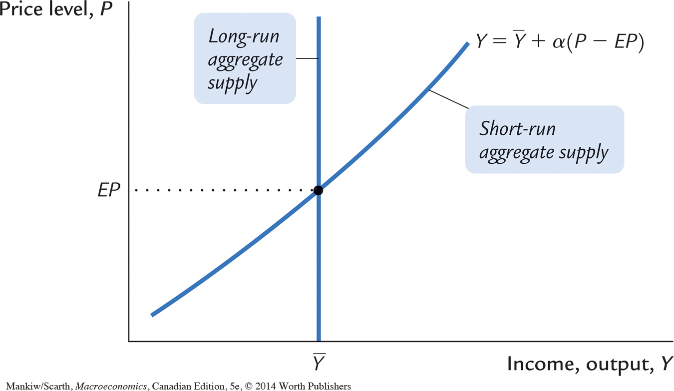
The two models of aggregate supply differ in their assumptions and emphases, but their implications for aggregate output are similar. Both can be summarized by the equation
This equation states that deviations of output from the natural level are related to deviations of the price level from the expected price level. If the price level is higher than the expected price level, output exceeds its natural level. If the price level is lower than the expected price level, output falls short of its natural level. Figure 13-1 graphs this equation. Notice that the short-run aggregate supply curve is drawn for a given expectation EP and that a change in EP would shift the curve.
Now that we have a better understanding of aggregate supply, let’s put aggregate supply and aggregate demand back together. Figure 13-2 uses our aggregate supply equation to show how the economy responds to an unexpected increase in aggregate demand attributable, say, to an unexpected monetary expansion. In the short run, the equilibrium moves from point A to point B. The increase in aggregate demand raises the actual price level from P1 to P2. Because people did not expect this increase in the price level, the expected price level remains at EP2 , and output rises from Y1 to Y2, which is above the natural level
. Thus, the unexpected expansion in aggregate demand causes the economy to boom.
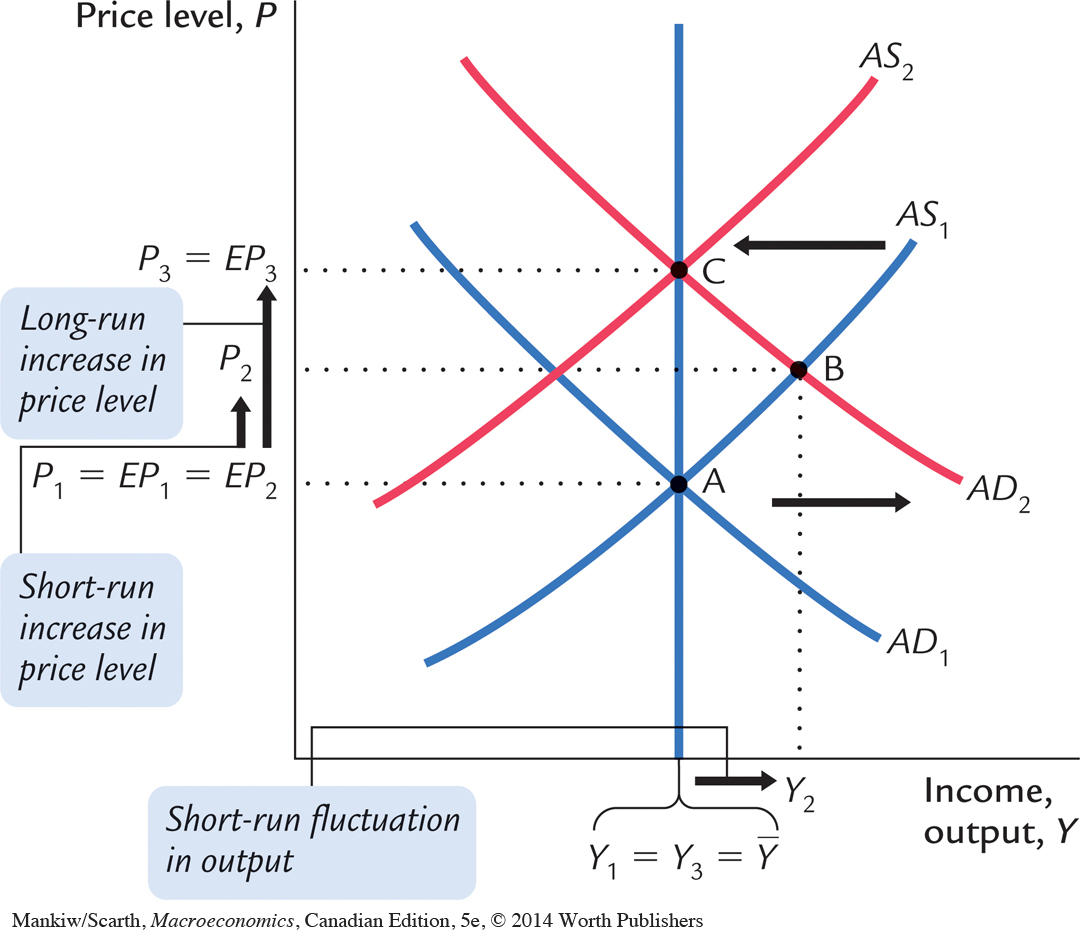
Yet the boom does not last forever. In the long run, the expected price level rises to catch up with reality, causing the short-run aggregate supply curve to shift upward. As the expected price level rises from EP2 to EP3, the equilibrium of the economy moves from point B to point C. The actual price level rises from P2 to P3, and output falls from Y2 to Y3. In other words, the economy returns to the natural level of output in the long run, but at a much higher price level.
433
This analysis shows an important principle, which holds for both models of aggregate supply: long-run monetary neutrality and short-run monetary nonneutrality are perfectly compatible. Short-run nonneutrality is represented here by the movement from point A to point B, and long-run monetary neutrality is represented by the movement from point A to point C. We reconcile the short-run and long-run effects of money by emphasizing the adjustment of expectations about the price level.