APPENDIX
A Big, Comprehensive Model
455
In the previous chapters, we have seen many models of how the economy works. When learning these models, it can be hard to see how they are related. Now that we have finished developing the model of aggregate demand and aggregate supply, this is a good time to look back at what we have learned. This appendix sketches a large comprehensive model that incorporates much of the theory we have already seen, including the classical theory presented in Part Two and the business cycle theory presented in Part Four. The notation and equations should be familiar from previous chapters. The goal is to put much of our previous analysis into a common framework to clarify the relationships among the various models.
The model has seven equations:
| Y = C(Y – T) + I(r) + G + NX(ϵ) | IS: Goods Market Equilibrium |
| M/P = L(i, Y) | LM: Money Market Equilibrium |
| NX(ϵ) = CF(r – r*) | Foreign Exchange Market Equilibrium |
| i = r + Eπ | Relationship Between Real and Nominal Interest Rates |
| ϵ = eP/P* | Relationship Between Real and Nominal Exchange Rates |
Y =  + α(P – EP)
 |
Aggregate Supply |
= (F ,
,  )
) |
Natural Level of Output |
These seven equations determine the equilibrium values of seven endogenous variables: output Y, the natural level of output  , the real interest rate r, the nominal interest rate i, the real exchange rate ϵ, the nominal exchange rate e, and the price level P.
There are many exogenous variables that influence these endogenous variables. They include the money supply M, government purchases G, taxes T, the capital stock K, the labour force L, the world price level P*, and the world real interest rate r*. In addition, there are two expectation variables: the expectation of future inflation Eπ and the expectation of the current price level formed in the past EP. As written, the model takes these expectations as exogenous, although additional equations could be added to make them endogenous.
Although mathematical techniques are available to analyze this seven-equation model, they are beyond the scope of this book. But this large model is still useful, because we can use it to see how the smaller models we have examined are related to one another. In particular, many of the models we have been studying are special cases of this large model. Let’s consider six special cases in particular. (A problem at the end of this section examines a few more.)
Special Case 1: The Classic Closed Economy
456
Suppose that EP = P, L(i, Y) = (1/V)Y and CF(r – r*) = 0. In words, these equations mean that expectations of the price level adjust so that expectations are correct, that money demand is proportional to income, and that there are no international capital flows. In this case, output is always at its natural level, the real interest rate adjusts to equilibrate the goods market, the price level moves parallel with the money supply, and the nominal interest rate adjusts one-for-one with expected inflation. This special case corresponds to the economy analyzed in Chapters 3 and 4.
Special Case 2: The Classic Small Open Economy
Suppose that EP = P, L(i, Y) = (1/V)Y, and CF(r – r*) is infinitely elastic. Now we are examining the special case when international capital flows respond greatly to any differences between the domestic and world interest rates. This means that r = r* and that the trade balance NX equals the difference between saving and investment at the world interest rate. This special case corresponds to the economy analyzed in Chapter 5.
Special Case 3: The Basic Model of Aggregate Demand and Aggregate Supply
Suppose that α is infinite and L(i, Y) = (1/V)Y. In this case, the short-run aggregate supply curve is horizontal, and the aggregate demand curve is determined only by the quantity equation. This special case corresponds to the economy analyzed in Chapter 9.
Special Case 4: The IS–LM Model
Suppose that α is infinite and CF(r – r*) = 0. In this case, the short-run aggregate supply curve is horizontal, and there are no international capital flows. For any given level of expected inflation Eπ, the level of income and interest rate must adjust to equilibrate the goods market and the money market. This special case corresponds to the economy analyzed in Chapter 10 and 11.
Special Case 5: The Mundell–Fleming Model with a Floating Exchange Rate
Suppose that α is infinite and CF(r – r*) infinitely elastic. In this case, the short-run aggregate supply curve is horizontal, and international capital flows are so great as to ensure that r = r*. The exchange rate floats freely to reach its equilibrium level. This special case corresponds to the first economy analyzed in Chapter 12.
Special Case 6: The Mundell–Fleming Model with a Fixed Exchange Rate
457
Suppose that α is infinite, CF(r – r*) is infinitely elastic, and the nominal exchange rate e is fixed. In this case, the short-run aggregate supply curve is horizontal, huge international capital flows ensure that r = r*, but the exchange rate is set by the central bank. The exchange rate is now an exogenous policy variable, but the money supply M is an endogenous variable that must adjust to ensure the exchange rate hits the fixed level. This special case corresponds to the second economy analyzed in Chapter 12.
You should now see the value in this big model. Even though the model is too large to be useful in developing an intuitive understanding of how the economy works, it shows that the different models we have been studying are closely related. In each chapter, we made some simplifying assumptions to make the big model smaller and easier to understand.
Figure 13-7 presents a schematic diagram that illustrates how various models are related. In particular, it shows how, starting with the mother of all models above, you can arrive at some of the models examined in previous chapters. Here are the steps:
Classical or Keynesian? You decide whether you want a classical special case (which occurs when EP = P or when α equals zero, so output is at its natural level) or a Keynesian special case (which occurs when α equals infinity, so the price level is completely fixed).
Closed or Open? You decide whether you want a closed economy (which occurs when the capital flow CF always equals zero) or an open economy (which allows CF to differ from zero).
Floating or Fixed? If you are examining a small open economy, you decide whether the exchange rate is floating (in which case the central bank sets the money supply) or fixed (in which case the central bank allows the money supply to adjust).
Fixed Velocity? If you are considering a closed economy with the Keynesian assumption of fixed prices, you decide whether you want to focus on the special case in which velocity is exogenously fixed.
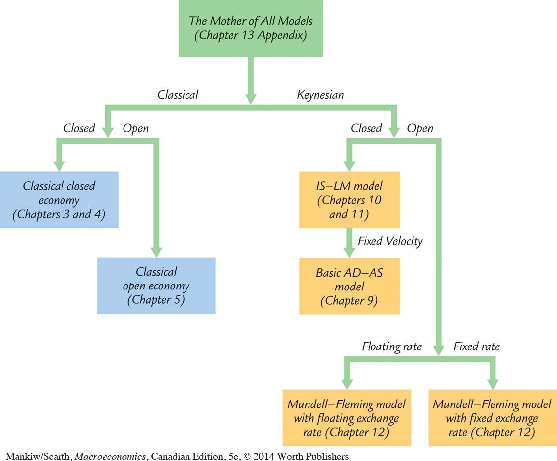
By making this series of modelling decisions, you move from the more complete and complex model to a simpler, more narrowly focused special case that is easier to understand and use.
When thinking about the real world, it is important to keep in mind all the models and their simplifying assumptions. Each of these models provides insight into some facet of the economy.