14.1 Elements of the Model
Before examining the components of the dynamic AD–AS model, we need to introduce one piece of notation: Throughout this chapter, the subscript t on a variable represents time. For example, Y is used to represent total output and national income, as it has been throughout this book. But now it takes the form Yt, which represents national income in time period t. Similarly, Yt+1 represents national income in period t – 1, and Yt+1 represents national income in period t + 1. This new notation will allow us to keep track of variables as they change over time.
Let’s now look at the five equations that make up the dynamic AD–AS model.
Output: The Demand for Goods and Services
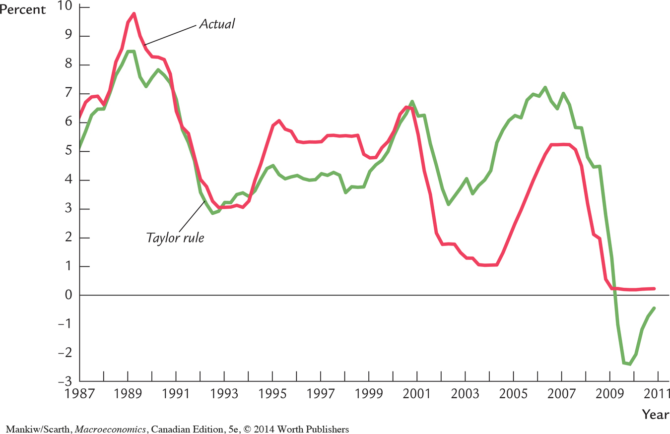
The demand for goods and services is given by the equation
where Yt is the total output of goods and services,  is the economy’s natural level of output, rt is the real interest rate, ϵt is a random demand shock, and α and ρ are parameters greater than zero. This equation is similar in spirit to the demand for goods and services equation in Chapter 3 and the IS equation in Chapter 10. Because this equation is so central to the dynamic AD–AS model, let’s examine each of the terms with some care.
The key feature of this equation is the negative relationship between the real interest rate rt and the demand for goods and services Yt. When the real interest rate increases, borrowing becomes more expensive, and saving yields a greater reward. As a result, firms engage in fewer investment projects, and consumers save more and spend less. Both of these effects reduce the demand for goods and services. (In addition, the high interest rate may attract foreign funds into the country so that our dollar might appreciate in foreign-exchange markets, causing net exports to fall, but for our purposes in this chapter these open-economy effects need not play a central role and can largely be ignored.) The parameter α tells us how sensitive demand is to changes in the real interest rate. The larger the value of α, the more the demand for goods and services responds to a given change in the real interest rate.
461
The first term on the right-hand side of the equation,
, implies that the demand for goods and services rises with the economy’s natural level of output. In most cases, we can simplify matters by taking this variable to be constant; that is,
will be assumed to be the same for every time period t. We will, however, examine how this model can incorporate long-run growth, represented by exogenous increases in
over time. A key piece of that analysis is apparent in this demand equation: as long-run growth makes the economy richer, the demand for goods and services grows proportionately.
The last term in the demand equation, ϵt, represents exogenous shifts in demand. Think of ϵt as a random variable—a variable whose values are determined by chance. It is zero on average but fluctuates over time. For example, if (as Keynes famously suggested) investors are driven in part by “animal spirits”—irrational waves of optimism and pessimism—those changes in sentiment would be captured by ϵt. When investors become optimistic, they increase their demand for goods and services, represented here by a positive value of ϵt. When they become pessimistic, they cut back on spending, and ϵt is negative.
The variable ϵt also captures changes in fiscal policy that affect the demand for goods and services. A temporary increase in government spending or a tax cut that stimulates consumer spending means a positive value of ϵt. A cut in government spending or a tax hike means a negative value of ϵt. Thus, this variable captures a variety of exogenous influences on the demand for goods and services.
Finally, consider the parameter ρ. From a mathematical perspective, ρ is just a constant, but it has a useful economic interpretation. It is the real interest rate at which, in the absence of any shock (ϵt = 0), the demand for goods and services equals the natural level of output. We can call ρ the natural rate of interest. Throughout this chapter, the natural rate of interest is assumed to be constant (although Problem 7 at the end of the chapter examines what happens if it changes). As we will see, in this model, the natural rate of interest plays a key role in the setting of monetary policy.
The Real Interest Rate: The Fisher Equation
The real interest rate in this model is defined as it has been in earlier chapters. The real interest rate rt is the nominal interest rate it minus the expected rate of future inflation Etπt+1. That is,
rt = it – Etπt+1.
This Fisher equation is similar to the one we first saw in Chapter 4. Here, Etπt+1 represents the expectation formed in period t of inflation in period t + 1. The variable rt is the ex ante real interest rate: the real interest rate that people anticipate based on their expectation of inflation.
A word on the notation and timing convention should clarify the meaning of these variables. The variables rt and it are interest rates that prevail at time t and, therefore, represent a rate of return between periods t and t + 1. The variable πt denotes the current inflation rate, which is the percentage change in the price level between periods t – 1 and t. Similarly, πt+1 is the percentage change in the price level that will occur between periods t and t + 1. As of time period t, πt+1 represents a future inflation rate and therefore is not yet known.
462
Note that the subscript on a variable tells us when the variable is determined. The nominal and ex ante real interest rates between t and t + 1 are known at time t, so they are written as it and rt. By contrast, the inflation rate between t and t + 1 is not known until time t + 1, so it is written as πt+1.
This subscript rule also applies when the expectations operator E precedes a variable, but here you have to be especially careful. As in previous chapters, the operator E in front of a variable denotes the expectation of that variable prior to its realization. The subscript on the expectations operator tells us when that expectation is formed. So Etπt+1 is the expectation of what the inflation rate will be in period t + 1 (the subscript on π) based on information available in period t (the subscript on E). While the inflation rate πt+1 is not known until period t + 1, the expectation of future inflation, Et πt+1, is known at period t. As a result, even though the ex post real interest rate, which is given by it – πt+1, will not be known until period t + 1, the ex ante real interest rate, rt = it – Etπt+1, is known at time t.
Inflation: The Phillips Curve
Inflation in this economy is determined by a conventional Phillips curve augmented to include roles for expected inflation and exogenous supply shocks. The equation for inflation is

This piece of the model is similar to the Phillips curve and short-run aggregate supply equation introduced in Chapter 13. According to this equation, inflation πt depends on previously expected inflation Et1+t, the deviation of output from its natural level (Yt –
), and an exogenous supply shock vt
Inflation depends on expected inflation because some firms set prices in advance. When these firms expect high inflation, they anticipate that their costs will be rising quickly and that their competitors will be implementing substantial price hikes. The expectation of high inflation thereby induces these firms to announce significant price increases for their own products. These price increases in turn cause high actual inflation in the overall economy. Conversely, when firms expect low inflation, they forecast that costs and competitors’ prices will rise only modestly. In this case, they keep their own price increases down, leading to low actual inflation.
The parameter ϕ, which is greater than zero, tells us how much inflation responds when output fluctuates around its natural level. Other things equal, when the economy is booming and output rises above its natural level, firms experience increasing marginal costs, and so they raise prices. When the economy is in recession and output is below its natural level, marginal cost falls, and firms cut prices. The parameter ϕ reflects both how much marginal cost responds to the state of economic activity and how quickly firms adjust prices in response to changes in cost.
463
In this model, the state of the business cycle is measured by the deviation of output from its natural level (Yt –
). The Phillips curves in Chapter 13 sometimes emphasized the deviation of unemployment from its natural rate. This difference is not significant, however. Recall Okun’s law from Chapter 2: Short-run fluctuations in output and unemployment are strongly and negatively correlated. When output is above its natural level, unemployment is below its natural rate, and vice versa. As we continue to develop this model, keep in mind that unemployment fluctuates along with output, but in the opposite direction.
The supply shock vt is a random variable that averages to zero but could, in any given period, be positive or negative. This variable captures all influences on inflation other than expectations of inflation (which is captured in the first term, Et–1πt) and short-run economic conditions [which are captured in the second term, ϕ(Yt –
). For example, if an aggressive oil cartel pushes up world oil prices, thus increasing overall inflation, that event would be represented by a positive value of vt. Similarly, if a hurricane destroys a number of the oil rigs in the Gulf of Mexico, raising world oil prices and causing inflation to rise, vt would also be positive. Similar events with effects moving in the opposite direction would make vt negative. In short, vt reflects all exogenous events that directly influence inflation.
Expected Inflation: Adaptive Expectations
As we have seen, expected inflation plays a key role in both the Phillips curve equation for inflation and the Fisher equation relating nominal and real interest rates. To keep the dynamic AD–AS model simple, we assume that people form their expectations of inflation based on the inflation they have recently observed. That is, people expect prices to continue rising at the same rate they have been rising. This is sometimes called the assumption of adaptive expectations. It can be written as
Etπt+1 = πt.
When forecasting in period t what inflation rate will prevail in period t + 1, people simply look at inflation in period t and extrapolate it forward.
The same assumption applies in every period. Thus, when inflation was observed in period t – 1, people expected that rate to continue. This implies that Et–1πt = πt–1.
This assumption about inflation expectations is admittedly crude. Many people are probably more sophisticated in forming their expectations. As we discussed in Chapter 13, some economists advocate an approach called rational expectations, according to which people optimally use all available information when forecasting the future. Incorporating rational expectations into the model is, however, beyond the scope of this book. (Moreover, the empirical validity of rational expectations is open to dispute.) The assumption of adaptive expectations greatly simplifies the exposition of the theory without losing many of the model’s insights.
The Nominal Interest Rate: The Monetary-Policy Rule
464
The last piece of the model is the equation for monetary policy. We assume that the central bank sets a target for the nominal interest rate it based on inflation and output using this rule:

In this equation, πt* is the central bank’s target for the inflation rate. (For most purposes, target inflation can be assumed to be constant, but we will keep a time subscript on this variable so we can examine later what happens when the central bank changes its target.) Two key policy parameters are θπ and θY, which are both assumed to be greater than zero. They indicate how much the central bank allows the interest rate target to respond to fluctuations in inflation and output. The larger the value of θπ, the more responsive the central bank is to the deviation of inflation from its target; the larger the value of θY, the more aggressive the central bank is in responding to the deviation of output from its natural level. Recall that ρ, the constant in this equation, is the natural rate of interest (the real interest rate at which, in the absence of any shock, the demand for goods and services equals the natural level of output). This equation tells us how the central bank uses monetary policy to respond to any situation it faces. That is, it tells us how the target for the nominal interest rate chosen by the central bank responds to macroeconomic conditions.
To interpret this equation, it is best to focus not just on the nominal interest rate it but also on the real interest rate rt. Recall that the real interest rate, rather than the nominal interest rate, influences the demand for goods and services. So, although the central bank sets a target for the nominal interest rate it, the bank’s influence on the economy works through the real interest rate rt. By definition, the real interest rate is rt = it – Etπt+1, but with our expectation equation Etπt+1 = πt, we can also write the real interest rate as rt = it – πt. According to the equation for monetary policy, if inflation is at its target (π = π*t) and output is at its natural level (Yt =
), the last two terms in the equation are zero, and so the real interest rate equals the natural rate of interest ρ. As inflation rises above its target (πt > πt*) or output rises above its natural level (Yt >
), the central bank takes steps to ensure that the real interest rate rises. And as inflation falls below its target (πt < πt*) or output falls below its natural level (Yt <
), the central bank engineers a reduction in the real interest rate.
At this point, one might naturally ask: what about the money supply? In previous chapters, such as Chapters 10 and 11, the money supply was typically taken to be the policy instrument of the central bank, and the interest rate adjusted to bring money supply and money demand into equilibrium. Here, we turn that logic on its head. The central bank is assumed to set a target for the nominal interest rate. It then adjusts the money supply to whatever level is necessary to ensure that the equilibrium interest rate (which balances money supply and demand) hits the target.
The main advantage of using the interest rate, rather than the money supply, as the policy instrument in the dynamic AD–AS model is that it is more realistic. Today, most central banks, including the Bank of Canada, set a short-term target for the nominal interest rate. Keep in mind, though, that hitting that target requires adjustments in the money supply. For this model, we do not need to specify the equilibrium condition for the money market, but we should remember that it is lurking in the background. When a central bank decides to change the interest rate, it is also committing itself to adjust the money supply accordingly.
465
CASE STUDY
The Taylor Rule
If you wanted to set interest rates to achieve low, stable inflation while avoiding large fluctuations in output and employment, how would you do it? This is exactly the question that the members of the governing council at the Bank of Canada must ask themselves every week. The short-term policy instrument that the Bank now sets is the overnight rate—the short-term interest rate at which banks make loans to one another. On eight pre-arranged dates each year, the Bank announces its current target for the overnight rate. The Bank’s overnight-loan traders are then told to conduct buy and sell orders so that the desired target is met.
The hard part of the Bank’s job is choosing the target for the overnight rate. Two general guidelines are clear. First, when inflation heats up, the overnight rate should rise. An increase in the interest rate will mean a smaller money supply and, eventually, lower investment, lower output, higher unemployment, and reduced inflation. Second, when real economic activity slows—as reflected in real GDP or unemployment—the overnight rate should fall. A decrease in the interest rate will mean a larger money supply and, eventually, higher investment, higher output, and lower unemployment. These two guidelines are represented by the monetary-policy equation in the dynamic AD–AS model.
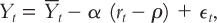
The Bank of Canada needs to go beyond these general guidelines, however, and determine its exact response to changes in inflation and real economic activity. Stanford University economist John Taylor has proposed the following rule for setting the similar interest rate in the United States—known as the federal funds rate1:
Nominal Federal Funds Rate = Inflation + 2.0 + 0.5 (Inflation – 2.0) + 0.5 (GDP gap).
The GDP gap is the percentage by which real GDP deviates from an estimate of its natural level. (For consistency with our dynamic AD–AS model, the GDP gap here is taken to be positive if GDP rises above its natural level and negative if it falls below it.)
According to the Taylor rule, the real federal funds rate—the nominal rate minus inflation—responds to inflation and the GDP gap. According to this rule, the real federal funds rate equals 2 percent when inflation is 2 percent and GDP is at its natural level. The first constant of 2 percent in this equation can be interpreted as an estimate of the natural rate of interest ρ, and the second constant of 2 percent subtracted from inflation can be interpreted as the Fed’s inflation target πt*. For each percentage point that inflation rises above 2 percent, the real federal funds rate rises by 0.5 percent. For each percentage point that real GDP rises above its natural level, the real federal funds rate rises by 0.5 percent. If inflation falls below 2 percent or GDP moves below its natural level, the real federal funds rate falls accordingly.
466
In addition to being simple and reasonable, the Taylor rule for monetary policy also resembles actual Fed behaviour in recent years. Figure 14-1 shows the actual nominal federal funds rate and the target rate as determined by Taylor’s proposed rule. Notice how the two series tend to move together. John Taylor’s monetary rule may be more than an academic suggestion. To some degree, it may be the rule that the Federal Reserve governors have been subconsciously following.
Canadian monetary policy is conducted in a similar fashion. As in the Taylor rule, the Bank of Canada’s target inflation rate has been 2 percent for a number of years. While the Bank has no similar explicit mandate concerning the output gap, Bank officials focus on keeping future inflation on target, and they know that—given the Phillips curve—this objective will not be met if the current output gap is allowed to become large. So the Bank reacts to variations in the output gap as well.
467
Researchers at the Bank of Canada have been debating whether it would be better if they targeted the price level, not just its rate of change through time—the inflation rate. Historical evidence has shown that—perhaps unintentionally—the Bank has actually delivered a time path for Canada’s price level that is without any long-term drift away from a growth path of 2 percent. So, as a matter of fact, Canada’s performance has been consistent with what would emerge with a price-level target. This is why, in the Appendix to Chapter 11, we investigated a macro model with the central bank being an interest-rate setter (as in the present chapter) but without the dynamics that we are dealing with here. By modelling the central bank as targeting the price level rather than its time derivative, the inflation rate, the analysis in the Chapter 11 Appendix was much simpler and not appreciably less realistic. One of the reasons for including the present chapter is to reassure readers that our Chapter 11 simplification avoiding explicit dynamics did not lead us astray. The more complete dynamic analysis in the present chapter is what provides this reassurance, and what permits readers to get a more complete glimpse of what current research-level analysis of monetary policy is actually like. 