14.3 Using the Model
Let’s now use the dynamic AD–AS model to analyze how the economy responds to changes in the exogenous variables. The four exogenous variables in the model are the natural level of output  , the supply shock vt, the demand shock ϵt, and the central bank’s inflation target πt*. To keep things simple, we will assume that the economy always begins in long-run equilibrium and is then subject to a change in one of the exogenous variables. Within each particular scenario, we also assume that the other exogenous variables are held constant.
Long-Run Growth
474
The economy’s natural level of output
changes over time because of population growth, capital accumulation, and technological progress, as discussed in Chapters 7 and 8. Figure 14-5 illustrates the effect of an increase in
. Because this variable affects both the dynamic aggregate demand curve and the dynamic aggregate supply curve, both curves shift. In fact, they both shift to the right by exactly the amount that
has increased. In the case of the dynamic aggregate supply curve, this is most easily appreciated by inverting its equation so that Yt, not πt, is on the left-hand side. When you do this, you will see that the coefficient on
is unity—just as it is in the equation of the dynamic aggregate demand curve.
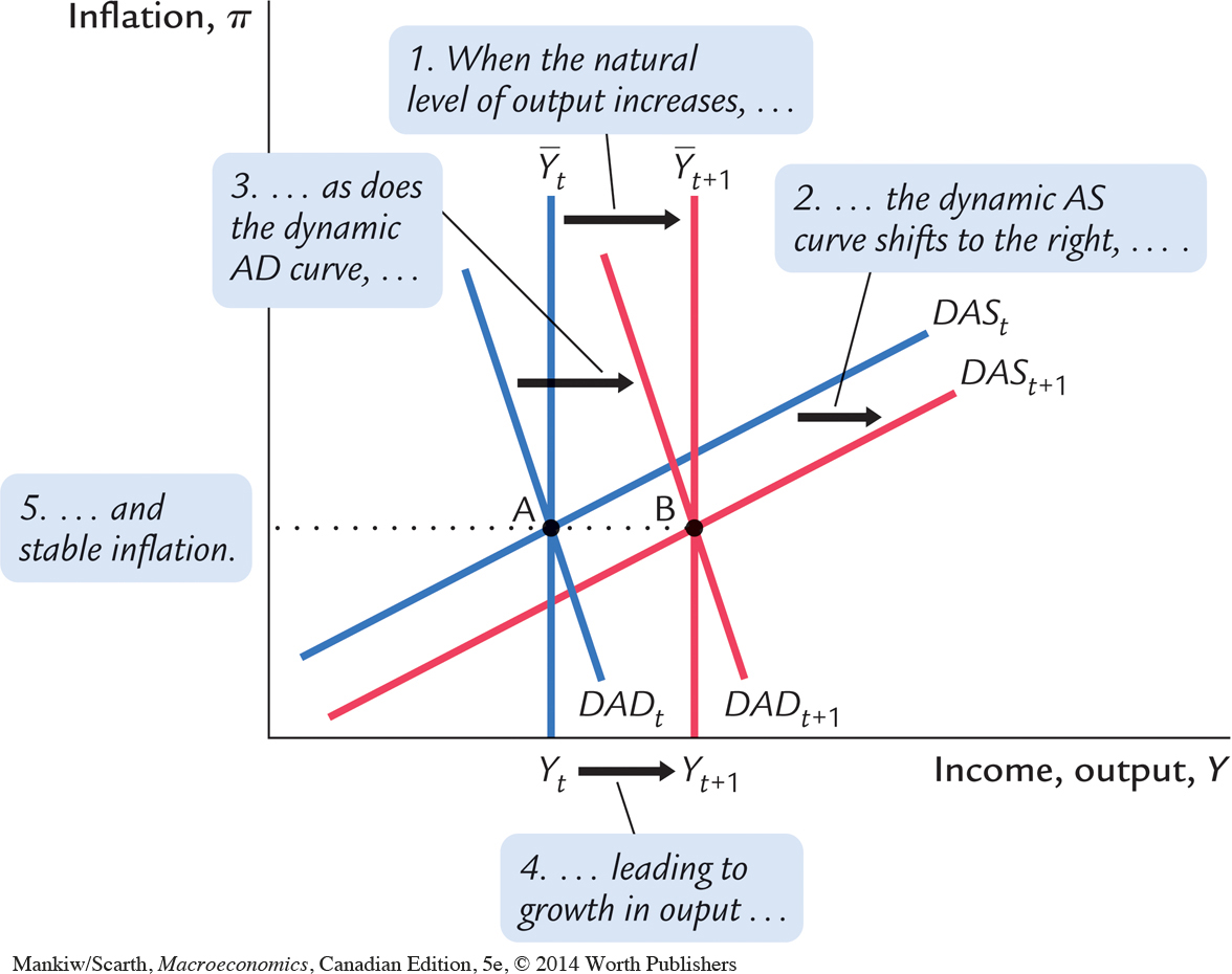 increases, both the dynamic aggregate demand curve and the dynamic aggregate supply curve shift to the right by the same amount. Output Yt increases, but inflation πt remains the same.
The shifts in these curves move the economy’s equilibrium in the figure from point A to point B. Output Yt increases by exactly as much as the natural level
. Inflation is unchanged.
The story behind these conclusions is as follows: When the natural level of output increases, the economy can produce a larger quantity of goods and services. This is represented by the rightward shift in the dynamic aggregate supply curve. At the same time, the increase in the natural level of output makes people richer. Other things equal, they want to buy more goods and services. This is represented by the rightward shift in the dynamic aggregate demand curve. The simultaneous shifts in supply and demand increase the economy’s output without putting either upward or downward pressure on inflation. In this way, the economy can experience long-run growth and a stable inflation rate.
A Shock to Aggregate Supply
475
Consider now a shock to aggregate supply. In particular, suppose that vt rises to 1 percent for one period and subsequently returns to zero. This shock to the Phillips curve might occur, for example, because a hurricane destroys some oil rigs, causing energy costs to rise and prices to be pushed up, or because new union agreements raise wages and, thereby, the costs of production. In general, the supply shock vt captures any event that influences inflation beyond expected inflation Et–1πt and current economic activity, as measured by Yt –
.
Figure 14-6 shows the result. In period t, when the shock occurs, the dynamic aggregate supply curve shifts upward from DASt–1 to DASt. To be precise, the curve shifts upward by exactly the size of the shock, which we assumed to be 1 percentage point. Because the supply shock vt is not a variable in the dynamic aggregate demand equation, the DAD curve is unchanged. Therefore, the economy moves along the dynamic aggregate demand curve from point A to point B. As the figure illustrates, the supply shock in period t causes inflation to rise to πt and output to fall to Yt.
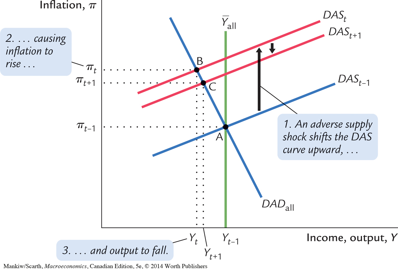
These effects work in part through the reaction of monetary policy to the shock. When the supply shock causes inflation to rise, the central bank responds by following its policy rule and raising nominal and real interest rates. The higher real interest rate reduces the quantity of goods and services demanded, which depresses output below its natural level. (This series of events is represented by the movement along the DAD curve from point A to point B.) The lower level of output dampens the inflationary pressure to some degree, so inflation rises somewhat less than the initial shock.
476
FYI
The Numerical Calibration and Simulation
The text presents some numerical simulations of the dynamic AD–AS model. When interpreting these results, it is easiest to think of each period as representing one year. We examine the impact of the change in the year of the shock (period t) and over the subsequent 12 years.
The simulations use these parameter values:

πt* = 2.0.
α = 1.0.
ρ = 2.0.
Φ = 0.25.
θπ = 0.5.
θY = 0.5.
Here is how to interpret these numbers. The natural level of output
is 100; as a result of choosing this convenient number, fluctuations in Yt –
can be viewed as percentage deviations of output from its natural level. The central bank’s inflation target πt* is 2 percent. The parameter α = 1.0 implies that a 1-percentage-point increase in the real interest rate reduces output demand by 1, which is 1 percent of its natural level. The economy’s natural rate of interest r is 2 percent. The Phillips curve parameter ϕ = 0.25 implies that when output is 1 percent above its natural level, inflation rises by 0.25 percentage point. The parameters for the monetary policy rule θπ = 0.5 and θY = 0.5 are those suggested by John Taylor and, as we saw earlier, are reasonable approximations of the behaviour of the actual central bank.
In all cases, the simulations assume a change of 1 percentage point in the exogenous variable of interest. Larger shocks would have qualitatively similar effects, but the magnitudes would be proportionately greater. For example, a shock of 3 percentage points would affect all the variables in the same way as a shock of 1 percentage point, but the movements would be three times as large as in the simulation shown.
The graphs of the time paths of the variables after a shock (shown in Figures 14-7, 14-9, and 14-11) are called impulse response functions. The word impulse refers to the shock, and “response function” refers to how the endogenous variables respond to the shock over time. These simulated impulse response functions are one way to illustrate how the model works. They show how the endogenous variables move when a shock hits the economy, how these variables adjust in subsequent periods, and how they are correlated with one another over time.
In the periods after the shock occurs, expected inflation is higher because expectations depend on past inflation. In period t + 1, for instance, the economy is at point C. Even though the shock variable vt returns to its normal value of zero, the dynamic aggregate supply curve does not immediately return to its initial position. Instead, it slowly shifts back downward toward its initial position DASt–1 as a lower level of economic activity reduces inflation and thereby expectations of future inflation. Throughout this process, output remains below its natural level.
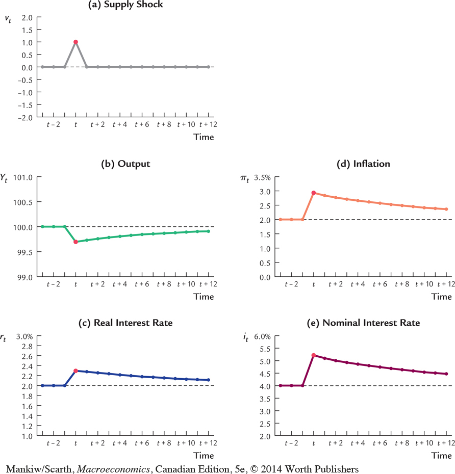
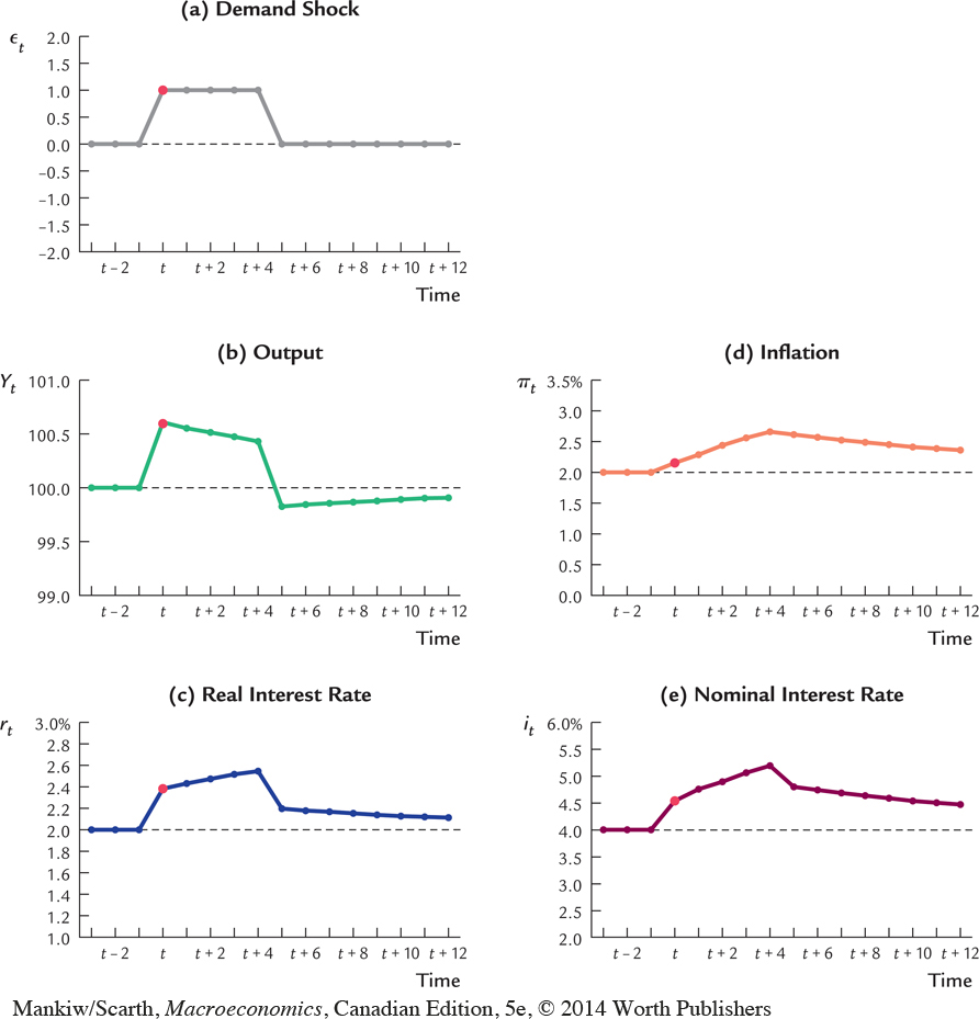
Figure 14-7 shows the time paths of the key variables in the model in response to the shock. (These simulations are based on realistic parameter values: see the nearby FYI box for their description.) As panel (a) shows, the shock vt spikes upward by 1 percentage point in period t and then returns to zero in subsequent periods. Inflation, shown in panel (d), rises by 0.9 percentage point and gradually returns to its target of 2 percent over a long period of time. Output, shown in panel (b), falls in response to the supply shock but also eventually returns to its natural level.
477
The figure also shows the paths of nominal and real interest rates. In the period of the supply shock, the nominal interest rate, shown in panel (e), increases by 1.2 percentage points, and the real interest rate, in panel (c), increases by 0.3 percentage points. Both interest rates return to their normal values as the economy returns to its long-run equilibrium.
These figures illustrate the phenomenon of stagflation in the dynamic AD–AS model. An adverse supply shock causes inflation to rise, which in turn increases expected inflation. As the central bank applies its rule for monetary policy and responds by raising interest rates, it gradually squeezes inflation out of the system, but only at the cost of a prolonged downturn in economic activity.
A Shock to Aggregate Demand
478
Now let’s consider a shock to aggregate demand. To be realistic, if the disturbance is to represent a major fiscal stimulus like the one introduced in 2009, the shock is assumed to persist over several periods. In particular, for our illustration, we suppose that ϵt = 1 for five periods and then returns to its normal value of zero. In addition to a major fiscal policy, the positive shock ϵt might represent, for example, a war that increases government purchases or a stock market bubble that increases wealth and thereby consumption spending. In general, the demand shock captures any event that influences the demand for goods and services for given values of the natural level of output
and the real interest rate rt.
Figure 14-8 shows the result. In period t, when the shock occurs, the dynamic aggregate demand curve shifts to the right from DADt–1 to DADt. Because the demand shock ϵt is not a variable in the dynamic aggregate supply equation, the DAS curve is unchanged from period t – 1 to period t. The economy moves along the dynamic aggregate supply curve from point A to point B. Output and inflation both increase.
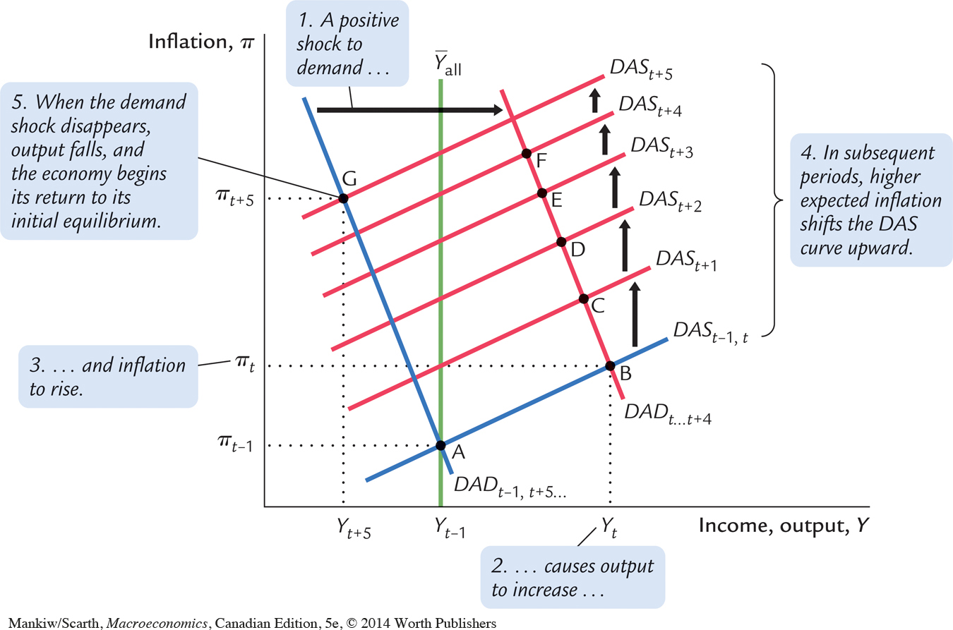
Once again, these effects work in part through the reaction of monetary policy to the shock. When the demand shock causes output and inflation to rise, the central bank responds by increasing the nominal and real interest rates. Because a higher real interest rate reduces the quantity of goods and services demanded, it partly offsets the expansionary effects of the demand shock.
In the periods after the shock occurs, expected inflation is higher because expectations depend on past inflation. As a result, the dynamic aggregate supply curve shifts upward repeatedly; as it does so, it continually reduces output and increases inflation. In the figure, the economy goes from point B in the initial period of the shock to points C, D, E, and F in subsequent periods.
In the sixth period (t + 5), the demand shock disappears. At this time, the dynamic aggregate demand curve returns to its initial position. However, the economy does not immediately return to its initial equilibrium, point A. The period of high demand has increased inflation and thereby expected inflation. High expected inflation keeps the dynamic aggregate supply curve higher than it was initially. As a result, when demand falls off, the economy’s equilibrium moves to point G, and output falls to Yt+5, which is below its natural level. The economy then gradually recovers, as the higher-than-target inflation is squeezed out of the system.
Figure 14-9 shows the time path of the key variables in the model in response to the demand shock. Note that the positive demand shock increases real and nominal interest rates. When the demand shock disappears, both interest rates fall. These responses occur because when the central bank sets the nominal interest rate, it takes into account both inflation rates and deviations of output from its natural level.
A Shift in Monetary Policy
479
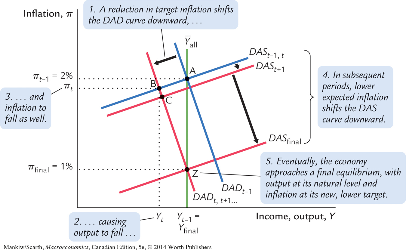
Suppose that the central bank decides to reduce its target for the inflation rate. Specifically, imagine that, in period t, πt* falls from 2 percent to 1 percent and thereafter remains at that lower level. Let’s consider how the economy will react to this change in monetary policy.
Recall that the inflation target enters the model as an exogenous variable in the dynamic aggregate demand curve. When the inflation target falls, the DAD curve shifts to the left, as shown in Figure 14-10. (To be precise, it shifts downward by exactly 1 percentage point.) Because target inflation does not enter the dynamic aggregate supply equation, the DAS curve does not shift initially. The economy moves from its initial equilibrium, point A, to a new equilibrium, point B. Output and inflation both fall.
 , and inflation ends at its new, lower target (πt*, t+1, . . . = 1 percent).
480
Monetary policy is, not surprisingly, key to the explanation of this outcome. When the central bank lowers its target for inflation, current inflation is now above the target, so the central bank follows its policy rule and raises real and nominal interest rates. The higher real interest rate reduces the demand for goods and services. When output falls, the Phillips curve tells us that inflation falls as well.
Lower inflation, in turn, reduces the inflation rate that people expect to prevail in the next period. In period t + 1, lower expected inflation shifts the dynamic aggregate supply curve downward, to DASt+1. (To be precise, the curve shifts downward by exactly the fall in expected inflation.) This shift moves the economy from point B to point C, further reducing inflation and expanding output. Over time, as inflation continues to fall and the DAS curve continues to shift toward DASfinal, the economy approaches a new long-run equilibrium at point Z, where output is back at its natural level (Yfinal =  ) and inflation is at its new lower target (πt*,t+1, . . . = 1 percent).
481
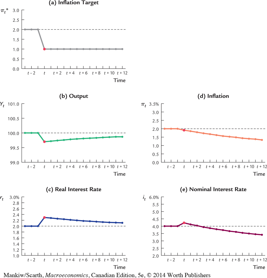
Figure 14-11 shows the response of the variables over time to a reduction in target inflation. Note in panel (e) the time path of the nominal interest rate it. Before the change in policy, the nominal interest rate is at its long-run value of 4.0 percent (which equals the natural real interest rate ρ of 2 percent plus target inflation π*t–1 of 2 percent). When target inflation falls to 1 percent, the nominal interest rate rises to 4.2 percent. Over time, however, the nominal interest rate falls as inflation and expected inflation fall toward the new target rate; eventually, it approaches its new long-run value of 3.0 percent. Thus, a shift toward a lower inflation target increases the nominal interest rate in the short run but decreases it in the long run.
482
We close with a caveat: Throughout this analysis we have maintained the assumption of adaptive expectations. That is, we have assumed that people form their expectations of inflation based on the inflation they have recently experienced. It is possible, however, that if the central bank makes a credible announcement of its new policy of lower target inflation, people will respond by altering their expectations of inflation immediately. That is, they may form expectations rationally, based on the policy announcement, rather than adaptively, based on what they have experienced. (We discussed this possibility in Chapter 13.) If so, the dynamic aggregate supply curve will shift downward immediately upon the change in policy, just when the dynamic aggregate demand curve shifts downward. In this case, the economy will instantly reach its new long-run equilibrium. By contrast, if people do not believe an announced policy of low inflation until they see it, then the assumption of adaptive expectations is appropriate, and the transition path to lower inflation will involve a period of lost output, as shown in Figure 14-11.