14.4 Two Applications: Lessons for Monetary Policy
483
So far in this chapter, we have assembled a dynamic model of inflation and output and used it to show how various shocks affect the time paths of output, inflation, and interest rates. We now use the model to shed light on the design of monetary policy.
It is worth pausing at this point to consider what we mean by the phrase “the design of monetary policy.” So far in this analysis, the central bank has had a simple role: it merely had to adjust the money supply to ensure that the nominal interest rate hit the target level prescribed by the monetary-policy rule. The two key parameters of that policy rule are θπ (the responsiveness of the target interest rate to inflation) and θY (the responsiveness of the target interest rate to output). We have taken these parameters as given without discussing how they are chosen. Now that we know how the model works, we can consider a deeper question: what should the parameters of the monetary policy rule be?
The Tradeoff Between Output Variability and Inflation Variability
Consider the impact of a supply shock on output and inflation. According to the dynamic AD–AS model, the impact of this shock depends crucially on the slope of the dynamic aggregate demand curve. In particular, the slope of the DAD curve determines whether a supply shock has a large or small impact on output and inflation.
This phenomenon is illustrated in Figure 14-12. In the two panels of this figure, the economy experiences the same supply shock. In panel (a), the dynamic aggregate demand curve is nearly flat, so the shock has a small effect on inflation but a large effect on output. In panel (b), the dynamic aggregate demand curve is steep, so the shock has a large effect on inflation but a small effect on output.
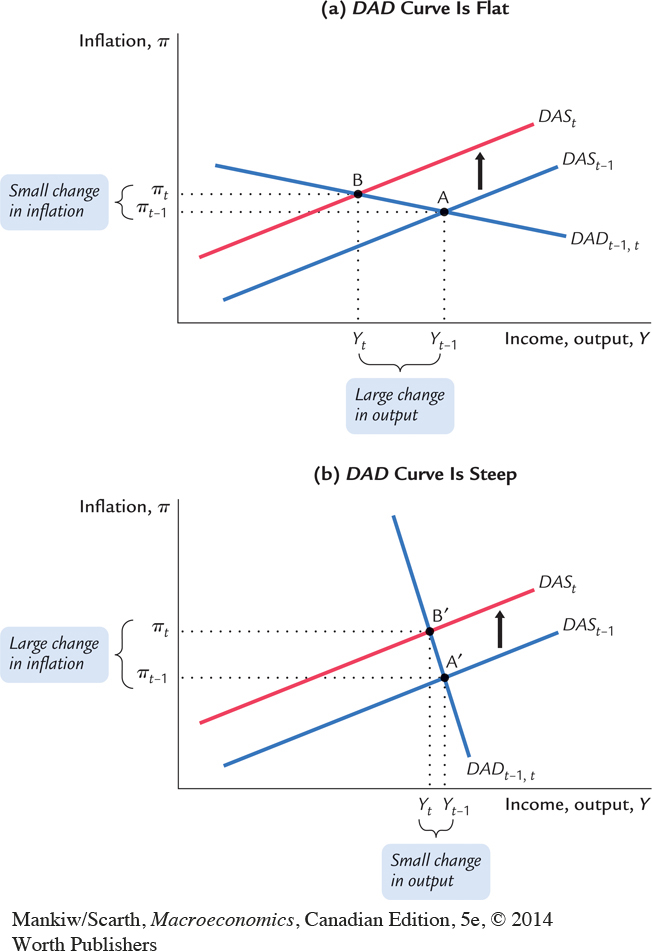
Why is this important for monetary policy? Because the central bank can influence the slope of the dynamic aggregate demand curve. Recall the equation for the DAD curve:

Two key parameters here are θπ and θY, which govern how much the central bank’s interest rate target responds to changes in inflation and output. When the central bank chooses these policy parameters, it determines the slope of the DAD curve and thus the economy’s short-run response to supply shocks.
484
On the one hand, suppose that, when setting the interest rate, the central bank responds strongly to inflation (θπ is large) and weakly to output (θY is small). In this case, the coefficient on inflation in the above equation is large. That is, a small change in inflation has a large effect on output. As a result, the dynamic aggregate demand curve is relatively flat, and supply shocks have large effects on output but small effects on inflation. The story goes like this: When the economy experiences a supply shock that pushes up inflation, the central bank’s policy rule has it respond vigorously with higher interest rates. Sharply higher interest rates significantly reduce the quantity of goods and services demanded, thereby leading to a large recession that dampens the inflationary impact of the shock (which was the purpose of the monetary policy response).
485
On the other hand, suppose that, when setting the interest rate, the central bank responds weakly to inflation (θπ is small) but strongly to output (θY is large). In this case, the coefficient on inflation in the above equation is small, which means that even a large change in inflation has only a small effect on output. As a result, the dynamic aggregate demand curve is relatively steep, and supply shocks have small effects on output but large effects on inflation. The story is just the opposite as before: Now, when the economy experiences a supply shock that pushes up inflation, the central bank’s policy rule has it respond with only slightly higher interest rates. This small policy response avoids a large recession but accommodates the inflationary shock.
In its choice of monetary policy, the central bank determines which of these two scenarios will play out. That is, when setting the policy parameters θπ and θY, the central bank chooses whether to make the economy look more like panel (a) or more like panel (b) of Figure 14-12. When making this choice, the central bank faces a tradeoff between output variability and inflation variability. The central bank can be a hard-line inflation fighter, as in panel (a), in which case inflation is stable but output is volatile. Alternatively, it can be more accommodative, as in panel (b), in which case inflation is volatile but output is more stable. It can also choose some position in between these two extremes.
One job of a central bank is to promote economic stability. There are, however, various dimensions to this charge. When there are tradeoffs to be made, the central bank has to determine what kind of stability to pursue. The dynamic AD–AS model shows that one fundamental tradeoff is between the variability in inflation and the variability in output.
Note that this tradeoff is very different from a simple tradeoff between inflation and output. In the long run of this model, inflation goes to its target, and output goes to its natural level. Consistent with classical macroeconomic theory, policymakers do not face a long-run tradeoff between inflation and output. Instead, they face a choice about which of these two measures of macro-economic performance they want to stabilize. When deciding on the parameters of the monetary-policy rule, they determine whether supply shocks lead to inflation variability, output variability, or some combination of the two.
CASE STUDY
The United States Fed Versus the European Central Bank
According to the dynamic AD–AS model, a key policy choice facing any central bank concerns the parameters of its policy rule. The monetary parameters θπ and θY determine how much the interest rate responds to macroeconomic conditions. As we have just seen, these responses in turn determine the volatility of inflation and output.
486
The U.S. Federal Reserve (Fed) and the European Central Bank (ECB) appear to have different approaches to this decision. The legislation that created the Fed states explicitly that its goal is “to promote effectively the goals of maximum employment, stable prices, and moderate long-term interest rates.” Because the Fed is supposed to stabilize both employment and prices, it is said to have a dual mandate. (The third goal—moderate long-term interest rates—should follow naturally from stable prices.) By contrast, the ECB says on its website that “the primary objective of the ECB’s monetary policy is to maintain price stability. The ECB aims at inflation rates of below, but close to, 2% over the medium term.” All other macroeconomic goals, including stability of output and employment, appear to be secondary. As far as its mandate is concerned, the Bank of Canada is very similar to the ECB, not the Fed.
We can interpret these differences in central bank mandates in light of our model. Compared to the Fed, the ECB seems to give more weight to inflation stability and less weight to output stability. This difference in objectives should be reflected in the parameters of the monetary-policy rules. To achieve its dual mandate, the Fed would respond more to output and less to inflation than the ECB would.
A case in point occurred in 2008 when the world economy was experiencing rising oil prices, a financial crisis, and a slowdown in economic activity. The Fed responded to these events by lowering interest rates from about 5 percent to a range of 0 to 0.25 percent over the course of a year. The ECB, facing a similar situation, also cut interest rates—but only later on. The ECB was less concerned about recession and more concerned about keeping inflation in check.
The dynamic AD–AS model predicts that, other things equal, the policy of the ECB should, over time, lead to more variable output and more stable inflation. Testing this prediction, however, is difficult for two reasons. First, because the ECB was established only in 1998, there is not yet enough data to establish the long-term effects of its policy. Second, and perhaps more important, other things are not always equal. Europe and the United States differ in many ways beyond the policies of their central banks, and these other differences may affect output and inflation in ways unrelated to differences in monetary-policy priorities. 
The Taylor Principle
How much should the nominal interest rate set by the central bank respond to changes in inflation? The dynamic AD–AS model does not give a definitive answer, but it does offer an important guideline.
Recall the equation for monetary policy:

According to this equation, a 1-percentage-point increase in inflation πt induces an increase in the nominal interest rate it of 1 + θπ percentage points. Because we assume that that θπ is greater than zero, whenever inflation increases, the central bank raises the nominal interest rate by an even larger amount.
487
Imagine, however, that the central bank behaved differently and, instead, increased the nominal interest rate by less than the increase in inflation. In this case, the monetary policy parameter θπ would be less than zero. This change would profoundly alter the model. Recall that the dynamic aggregate demand equation is:

If θπ is negative, then an increase in inflation would increase the quantity of output demanded, and the dynamic aggregate demand curve would be upward sloping.
An upward-sloping DAD curve leads to unstable inflation, as illustrated in Figure 14-13. Suppose that in period t there is a one-time positive shock to aggregate demand. That is, for one period only, the dynamic aggregate demand curve shifts to the right, to DADt; in the next period, it returns to its original position. In period t, the economy moves from point A to point B. Output and inflation rise. In the next period, because higher inflation has increased expected inflation, the dynamic aggregate supply curve shifts upward, to DASt+1. The economy moves from point B to point C. But because we are assuming in this case that the dynamic aggregate demand curve is upward sloping, output remains above the natural level, even though demand shock has disappeared. Thus, inflation rises yet again, shifting the DAS curve farther upward in the next period, moving the economy to point D. And so on. Inflation continues to rise with no end in sight.
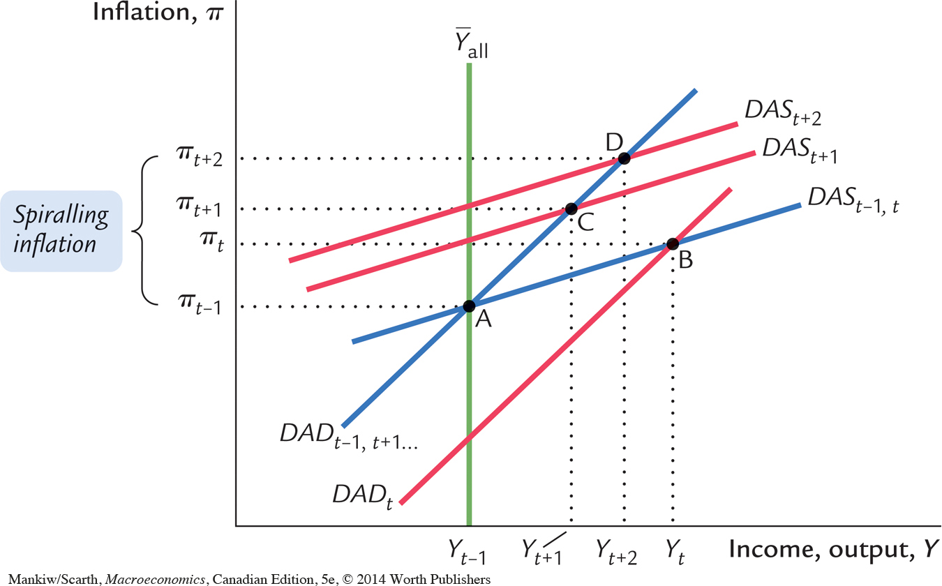
488
The economic intuition may be easier to understand than the geometry. A positive demand shock increases output and inflation. If the central bank does not increase the nominal interest rate sufficiently, the real interest rate falls. A lower real interest rate increases the quantity of goods and services demanded. Higher output puts further upward pressure on inflation, which in turn lowers the real interest rate yet again. The result is inflation spiralling out of control.
The dynamic AD–AS model leads to a strong conclusion: For inflation to be stable, the central bank must respond to an increase in inflation with an even greater increase in the nominal interest rate. This conclusion is sometimes called the Taylor principle, after economist John Taylor, who emphasized its importance in the design of monetary policy. Most of our analysis in this chapter assumed that the Taylor principle holds (that is, we assumed that θπ > 0). We can see now that there is good reason for a central bank to adhere to this guideline.
CASE STUDY
What Caused the Great Inflation?
In the 1970s, inflation in all western countries, including Canada, got out of hand. As we saw in previous chapters, the inflation rate during this decade reached double-digit levels. Rising prices were widely considered the major economic problem of the time. Beginning in the early 1980s, contractionary monetary policy was used to eventually bring inflation back under control. Then we had low and stable inflation for the next quarter century.
The dynamic AD–AS model offers a new perspective on these events. According to research by monetary economists Richard Clarida, Jordi Gali, and Mark Gertler, the key is the Taylor principle. Clarida and colleagues examined the U.S. data on interest rates, output, and inflation and estimated the parameters of the monetary policy rule. They found that the U.S. monetary policy obeyed the Taylor principle after 1980, whereas earlier monetary policy did not. In particular, the parameter θπ was estimated to be 0.72 after 1980, close to Taylor’s proposed value of 0.5, but it was –0.14 during the 1960s and 1970s.2 The negative value of θπ during the earlier era means that monetary policy did not satisfy the Taylor principle.
489
This finding suggests a potential cause of the great inflation of the 1970s. When the U.S. economy was hit by demand shocks (such as government spending on the Vietnam War) and supply shocks (such as the OPEC oil-price increases), the Fed raised nominal interest rates in response to rising inflation but not by enough. Therefore, despite the increase in nominal interest rates, real interest rates fell. The insufficient monetary response not only failed to squash the inflationary pressures but actually exacerbated them. The problem of spiralling inflation was not solved until the monetary-policy rule was changed to include a more vigorous response of interest rates to inflation.
An open question is why policymakers were so passive in the earlier era. Here are some conjectures from Clarida, Gali, and Gertler:
Why is it that during the pre-1979 period the Federal Reserve followed a rule that was clearly inferior? Another way to look at the issue is to ask why it is that the Fed maintained persistently low short-term real rates in the face of high or rising inflation. One possibility . . . is that the Fed thought the natural rate of unemployment at this time was much lower than it really was (or equivalently, that the output gap was much smaller). . . .
Another somewhat related possibility is that, at that time, neither the Fed nor the economics profession understood the dynamics of inflation very well. Indeed, it was not until the mid-to-late 1970s that intermediate textbooks began emphasizing the absence of a long-run tradeoff between inflation and output. The ideas that expectations may matter in generating inflation and that credibility is important in policymaking were simply not well established during that era. What all this suggests is that in understanding historical economic behaviour, it is important to take into account the state of policymakers’ knowledge of the economy and how it may have evolved over time.