16.1 The Size of the Government Debt
Let’s begin by putting the government debt in perspective. As this book went to press, the debt of the Canadian federal government was about $600 billion. If we divide this number by 34 million, roughly the number of people in Canada at the time, we find that each person’s share of the government debt was about $17,650. Obviously, this is not a trivial number—few people sneeze at $17,650. Yet if we compare this debt to the roughly $1.5 million a typical person will earn over his or her working life, the government debt does not look like the catastrophe it is sometimes made out to be.
One way to judge the size of a government’s debt is to compare it to the amount of debt other countries have accumulated. Table 16-1 shows the amount of government debt for 28 major countries expressed as a percentage of each country’s GDP. On the top of the list are the heavily indebted countries of Greece, Japan, and Italy, which have accumulated a debt that exceeds annual GDP. At the bottom are Australia and Switzerland, which have accumulated relatively small debts. Canada is in the middle of the pack. By international standards, Canadian federal and provincial governments, taken as a group, are neither especially profligate nor especially frugal. (The table shows only federal government debt.)
| Country | Government Debt as a Percentage of GDP |
| Greece | 133.1 |
| Japan | 127.6 |
| Italy | 100.2 |
| Belgium | 80.4 |
| Portugal | 75.8 |
| United States | 73.8 |
| France | 62.7 |
| United Kingdom | 61.7 |
| Germany | 51.5 |
| Spain | 45.6 |
| Netherlands | 37.7 |
| Canada | 33.6 |
| Australia | 4.9 |
| Switzerland | 0.4 |
|
Source: OECD Economic Outlook. Data are net financial liabilities as a percent of GDP for 2011. |
|
|---|---|
Over the course of Canadian history, the indebtedness of the federal government has varied substantially. Figure 16-1 shows the ratio of the federal debt to GDP since 1925. What explains this variation?
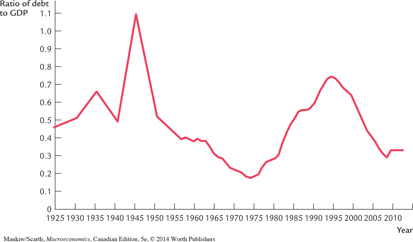
Focusing on just the Canadian federal government, national debt is the sum total of all the annual budget deficits incurred since confederation in 1867. That debt reached the $600 billion mark in 2012, and one-quarter of that total has been added since the 2008 recession! Since the Great Depression of the 1930s involved a much larger reduction in economic activity, the federal debt shot up during both that period, and during World War II, as Figure 16-1 shows. These developments have not been interpreted as government mismanagement, however, because people have reasoned that the government had no choice but to get involved in these crises. Most people think that because future generations have benefited from the freedom that the war ensured, it is only fair that they shoulder some of the burden. Issuing debt during the war, therefore, was the government’s way of spreading some of the costs to future generations.
537
Following the war, the federal government’s debt–GDP ratio was 110 percent. By 1970, it was less than 20 percent. The debt ratio was brought under control in three main ways. First, the government ran budget surpluses for a number of years in the 1945–1970 period, and in each of those years the debt was decreased by the amount of the surplus. Second, Canada enjoyed a long period of rapid economic growth. With real GDP growing briskly, the ratio of the outstanding debt to GDP shrank at a rapid rate. Finally, during the Korean War period in the early 1950s, and during the 1965–1980 period, Canada’s inflation rate reduced the real value of the debt by a significant amount. Unexpected inflation is simply a gradual (some would say “civilized”) way for a country to default on some of its debt.
By 1994, the federal debt ratio had climbed back up to 73 percent. There were two main reasons for this dramatic reversal of the postwar trend. First, Canada’s average growth rate for real GDP had been lower since the mid-1970s, when most Western countries began suffering from a slowdown in productivity growth. Second, the government simply overspent. The federal government ran a deficit every year between 1971 and 1998.
538
Broadly speaking, there are three reasons why many were concerned about the resulting increase in debt. First, Canadians were more indebted to foreigners. As a proportion of GDP, Canada’s net foreign debt (including all forms, not just government debt) was almost 50 percent in 1994. This put Canada in first place among G7 countries in foreign debt standings. (The second- and third-place finishers were Italy at 12 percent and the United States at 10 percent.) Just to pay the interest on that debt, Canadians had to give up 4.5 percent of GDP in 1994. On average, it is un-realistic to expect Canada’s economy to grow at that rate in real terms, so the prospects for an improvement in the Canadian standard of living were bleak. Second, many regard debt as worrisome because it may lead to further tax increases in order to pay for the interest. The tax–GDP ratio in Canada increased from 31.5 percent in 1980 to 37.5 percent in 1993, and despite higher taxes, federal debt service costs rose from 20 percent of tax revenue to 32 percent of revenue over this same period. Finally, the existence of the debt raises issues of equity. Some regard it as immoral that one generation “spends beyond its means,” thereby lowering the standard of living for future generations through such mechanisms as reduced government programs.
539
During the middle of the 1990s, the federal government started to get its budget deficit under control. A combination of spending cuts, rising taxes, and rapid economic growth caused the ratio of debt to GDP to stabilize and decline by about 10 percentage points by the end of the century. Our experience during most of the first decade of the new century tempted some observers to think that exploding government debt is a thing of the past. But as the 2009 recession hit, rising unemployment meant that the government’s tax collections shrunk and, at the same time, the stimulus package involved higher government spending. Both these developments caused the deficit, and therefore the accumulated debt, to start rising again. As the following case study suggests, it will likely take several more years for the resulting temporary rise in the debt-to-GDP ratio to be overcome. It is important that the debt ratio be put back on its previous downward trend, since some increase in this measure is likely to reappear in the years to come, as the aging baby boom generation withdraws from the labour force and demands increased health and pension benefits during their retirement.
CASE STUDY
Canadian Deficits and Debt: Past, Present, and Future
As noted earlier, between 1973 and 1993 our federal government debt ratio rose dramatically—by 50 percentage points. The Trudeau Liberals were in power for the first 10 years of this period, and the Mulroney Conservatives took over for the second half of this episode. As the size of the budget deficits grew during the Trudeau years, the Conservatives were adamant that they would stop the rise in debt if given the chance. Indeed, the Conservatives did run a more contractionary policy. Why did the debt ratio continue to explode nonetheless? When the Liberals took office again in 1993, why did they succeed in reversing the trend in the debt ratio—when the Conservatives had failed? To answer these questions, we need to understand the basic accounting relationships of deficits and debt.
The primary deficit is the excess of the government’s program spending over its tax revenue. Program spending is all government expenditure except interest payments. The overall deficit is the primary deficit plus the government’s interest payment obligations on its outstanding debt. To reduce the outstanding debt, the government must run an overall surplus, and this, in turn, requires a primary surplus that exceeds the existing interest payment obligations. As a first step, then, the government must eliminate its primary deficit. While this first step is not sufficient to reduce Canada’s national debt, you might think that it would be enough to eliminate the explosive growth in the ratio of the debt to GDP. History suggests that this is not the case. Brian Mulroney’s Conservative government maintained an average primary balance of zero, and was therefore much more prudent than the Trudeau Liberals, who averaged a sizable primary deficit. Despite this effort by the Conservatives, the deficit and debt problem worsened during their term of office. To appreciate why, let’s carefully distinguish the primary deficit, the overall deficit, the debt, and the debt ratio.
540
Letting D and B stand for the government’s deficit and the stock of outstanding bonds, respectively, we can summarize the key relationships as follows. The deficit is the excess of government spending over tax revenue (the primary deficit, G − T) plus interest payments on the outstanding bonds, rB:
D = G – T + rB.
The national debt increases by the size of the current deficit:
ΔB = D.
Using lowercase letters to stand for the ratio of each item to GDP (i.e., g = G/Y, t = T/Y, d = D/Y, and b = B/Y), then the deficit ratio is
d = g – t + rb,
and the increase in the debt ratio is
Δb = d – nb,
where n stands for the long-run average growth rate in output (which takes place because of productivity increases and population growth). This last relationship may require further explanation. Since b = B/Y, b rises whenever its numerator grows more than its denominator does. Thus,
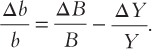
If Y grows at rate n (ΔY/Y = n) and the bond stock grows by the size of the deficit (ΔB = D) this relationship can be rewritten as
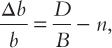
or
Δb = d – nb.
If the government sets the primary deficit ratio at some target value, it is setting (g – t) as an exogenous constant. The implications for the debt ratio can then be seen by eliminating d from our two key relationships:
Δb = (g – t) + (r – n)b.
Consider the Conservatives’ policy of setting (g – t) at zero. This relationship says that the debt ratio must forever rise—Δb is forever positive—if r exceeds n. That is, the debt ratio rises without bound if the interest rate the government pays on government bonds (the growth rate for the numerator of the debt ratio) exceeds the economy’s underlying average growth rate (the growth rate for the denominator of the debt ratio).
541
Since r exceeded n throughout the 1970s and 1980s, it is not surprising that Canada’s debt ratio rose inexorably, despite the Conservatives’ success in keeping (g – t) at zero.
The economy’s average growth rate exceeded interest rates during the 1950s and 1960s in Canada, when such factors as the postwar reconstruction of industry, the shift of population to the cities, and the development of Canada’s natural resources made growth particularly high. Given this temporary excess of n over r and the fact that the federal government often ran budget surpluses, it is not surprising that the debt ratio fell during these years (as shown in Figure 16-1). But considering long-run average values, we must realize that r exceeds n, so it is impossible to grow out of the debt problem by keeping the primary deficit at zero.1
When the Liberals took over in 1993, they switched to targeting the overall deficit ratio instead of targeting just the primary deficit ratio. Could we have expected this policy to have greater success in controlling the debt ratio?
The Liberal policy involved switching the exogenous and endogenous variables. Under the previous regime, (g – t) was exogenous and d was endogenous. The Liberals’ plan made d exogenous, and to accomplish this, they had to allow either g or t to become endogenous. Since their plan accomplished most of the deficit reduction through expenditure cuts, not tax increases, we take g as the endogenous variable in the following illustration.
Using a subscript of –1 to stand for previous period’s values, the debt-ratio growth equation can be rewritten as
b = (1 – n)b–1 + d
This debt-ratio growth equation says that the value of this period’s debt ratio is equal to the value of last period’s debt ratio plus the adjustments that indicate how both the numerator and the denominator of the debt ratio have grown over the period. The numerator has grown by the size of the deficit, and the denominator has grown by the economy’s rate of growth. The debt-ratio growth equation involves both these adjustments in ratio terms.
If d is an exogenous constant, the debt-ratio growth equation states that b cannot keep growing forever. Except for the constant d, this year’s debt ratio is just a fraction, (1 – n) of last period’s value. So the Liberal plan had to work. It involved the government’s “making room” in its budget by cutting programs by whatever was necessary to meet both the interest payment obligations and the overall deficit target. This policy succeeded, but it involved more pain in terms of lost programs.
To illustrate the magnitude of these cutbacks, Table 16-2 presents a simulation of the Liberal policy. The simulation starts with values for the deficit ratio (d = 0.06), the tax ratio (t = 0.17), the debt ratio (b = 0.70), the program spending ratio (g = 0.178), and the interest rate (r = 0.075), which represent what the Liberals inherited in 1993. These values satisfy the budget identity
d = g – t + rb.
| Fiscal Year | Deficit/GDP (d) | Debt/GDP (b) | Spending/GDP (g) | |
| 1993–1994 | 0.06 | 0.72 | 0.178 | |
| 1994–1995 | 0.05 | 0.73 | 0.166 | |
| 1995–1996 | 0.04 | 0.73 | 0.155 | |
| 1996–1997 | 0.03 | 0.72 | 0.145 | |
| 1997–1998 | 0 | 0.68 | 0.128 | |
| 1998–1999 | 0 | 0.64 | 0.130 | |
| 1999–2000 | –0.01 | 0.60 | 0.123 | |
| 2000–2001 | –0.01 | 0.56 | 0.126 | |
| 2001–2002 | –0.01 | 0.52 | 0.132 | |
| 2002–2003 | –0.01 | 0.48 | 0.129 | |
| 2003–2004 | –0.01 | 0.44 | 0.131 | |
| 2004–2005 | –0.01 | 0.41 | 0.134 | |
| 2005–2006 | –0.01 | 0.37 | 0.130 | |
| 2006–2007 | –0.01 | 0.34 | 0.131 | |
| 2007–2008 | –0.01 | 0.31 | 0.133 | |
| 2008–2009 | 0.003 | 0.29 | 0.126 | |
| 2009–2010 | 0.036 | 0.33 | 0.156 | |
| 2010–2011 | 0.020 | 0.33 | 0.144 | |
| 2011–2012 | 0.015 | 0.33 | 0.138 | |
| 2012–2013 | 0.014 | 0.33 | 0.138 |
542
From this starting position, the simulation involves an annual growth rate for GDP of 5.5 percent (n = 0.055). While actual history involved year-to-year variation in GDP growth, we simplify by taking just the average trend (3.5 percent real growth plus 2.0 percent inflation). We focus first on the top two sections of Table 16-2 (covering 1993–1999 when the government eliminated its deficit, and 1999–2008 when the government ran a surplus each year equal to roughly one percent of GDP each year.) To use the two budget accounting identities in a simulation, we need to make two more assumptions designed to reflect actual history. We insert representative values for the interest rate and the tax rate. In the former case, the 7.5 percent value is involved for the first four years, then, to reflect the general decline in interest rates through the following period, we insert 6.5 percent for four years, 6.0 percent for the next four years, and then 5 percent for three years. For the tax ratio, the 17 percent figure is assumed until the end of the 1996–1997 fiscal year; a slightly higher value, 17.5 percent, is assumed after that to reflect the fact that the government did adjust policy by approximately this amount for five years. Then, in the 2002–2008 period, the tax rate is 17 percent for three years and then 16 percent for three years—again to reflect the fact that the government cut tax rates during this period.
543
The second column in the table indicates the deficit ratio that the government imposed during each fiscal year that followed. We used the b+1 = (1 – n)b + d equation to generate the third-column entry (the next year’s debt ratio), and we used the g = d + t – rb equation to calculate the fourth-column entry (what had to happen to program spending to meet the deficit-ratio target).
Despite our simplifications, we see that the basic accounting identities do an excellent job of simulating history. They show the debt ratio falling by 40 percentage points to 31 percent by the end of the 2007–2008 fiscal year. This figure matches the true outcome of 30 percent very closely. The same can be said for the fourth column in the table. It indicates that dramatic spending cuts were needed to achieve this debt reduction. As a proportion of GDP, program spending had to be cut by a massive 5 percentage points of GDP in the first five years of this fiscal retrenchment exercise. And a decade later, the program spending ratio could recover by just one of these five percentage points. So, although the Liberals did get control of the debt ratio, this long-term gain resulted in a lot of short-term pain for those who depended on these government programs.
As just noted, after bottoming out in the fourth year of the deficit reduction period, the program spending ratio began to recover. The rise in program spending is widely referred to as the “fiscal dividend.” A fiscal dividend exists during a period of debt reduction because new room is created in the budget as the debt ratio falls. Lower debt means that the government has lower interest payment obligations, and the government can then use these funds to raise program spending, reduce taxes, or pay down debt. In the table, to match the government’s actual choices, we have assumed that the government chooses a combination of increased spending and debt reduction (budget surpluses).
How big is the “fiscal dividend” likely to be in the long run? To answer this question, we consider the budgetary implications of reducing the debt ratio by 50 percentage points—that is, back to the level of the early 1970s. The interest payments term in the budget identity, rb, would fall by rΔb, and for a 6 percent interest rate, that’s (0.06)(0.5) = 0.03. Thus, there would be 3 percentage points of GDP new room in the budget. Further, it is important to consider the full-equilibrium version of the Δb = d – nb equation. In full equilibrium, Δb = 0, so d = nb. If we settle on a full equilibrium with a 20 percent debt ratio, this relationship and a 5.5 percent growth rate imply that d = (0.055)(.2) = 0.011. Thus, moving from a balanced budget (which characterized the Canadian situation when the fiscal dividend debate began) to a full equilibrium involving a 20 percent debt ratio requires an increase in the deficit ratio of 1.1 percentage point. (d increases from 0 to 0.011.) Thus, the overall fiscal dividend in the long run is 4.1 percentage points of GDP.
To put this in perspective, it is worth noting that the entire federal personal income tax system raises just 8 percent of GDP. Thus, as long as debt reduction is part of our fiscal plan, the fiscal dividend will be enough to cut income taxes in half! (We are not suggesting that tax cuts are better than spending increases; this illustration is intended just to show the dramatic magnitude of what can accompany debt reduction.)
544
Of course, the debt ratio can gradually approach any target number, like 20 percent, whether we balance the budget or run surpluses in the short run. The choice between these two options concerns the distribution of costs and benefits over time. Relative to balanced budgets, surpluses involve short-term pain for long-term gain. We postpone receiving the fiscal dividend, but we reach the full magnitude of the benefits faster. Why should we be concerned about how long this takes?
To answer this question, many people focus on the aging of the population. With the oldest group within the large baby-boom generation starting retirement in 2011, and with increases in life expectancy generally, the proportion of the Canadian population that is over 65 years of age will double over the first 30 years of the present century. This fact will put a strain on our public pension and health-care systems (since most health-care expenses occur in older age). The Auditor General has estimated that the government will need at least 4 percentage points of GDP—beyond what is now spent—to maintain these programs. And surely the government will face other challenges. To mention just three, there are widespread demands (and government promises) for significant tax relief, there is the growing problem of rising income inequality (see the appendix to Chapter 6), and the need to address environmental and climate- change concerns. Even ignoring these and all other demands on the public purse, the fiscal dividend may be just barely big enough to cover the aging problem.
These facts indicate that we will almost certainly have to return to a series of years involving budget deficits in the longer-term future. To keep this development from pushing debt levels to new heights, many feel that we have a limited number of years to get the debt ratio down if we are to make room for the future rise that will occur when the demographic shock hits.
The government has accepted this analysis. The federal finance department funded a conference in 2003, asking participants to provide guidance concerning what target the government should identify for the ratio of the outstanding debt to GDP. Research presented at the conference showed that a target of between 20 and 25 percent—reached within 10 years—would be necessary if we want to limit the threat to the growth in average living standards posed by the aging of the baby boomer generation.2 In the 2004 Budget, the government adopted this very target. The 2005 Economic Update of Finance Canada contained the following statements:
With the aging of Canada’s population, the country will face increases in aging-related expenditures, such as elderly benefits and health care. In order to meet these future pressures, it is critical that the federal government maintain a strong focus on fiscal discipline and debt reduction over the next several years, before the major impacts of population aging are felt.
In the 2004 budget, the Government set a long-run goal of reducing the debt-to-GDP ratio to 25 per cent by 2014–15.
In 2013, the government reiterated its target of 25% but revised the target date to 2021.
545
By focusing on the last year before the financial crisis and recession—the 2007–2008 fiscal year—we can see that the government was well on its way to reaching this long-term target for the debt ratio within the desired time frame. But then the 2008–2009 recession hit. To illustrate how much this development limited the government’s ability to reach its longer-term debt-reduction objective, we have extended our reporting in Table 16-2 to include five more fiscal years. In this section of the table, we include the actual data for all four columns, as reported in the Fall 2012 Fiscal Update issued by Finance Canada. As we can see, the recession caused the long-term decline in the debt ratio to be reversed. Instead of falling by another 13 percentage points as it did in the previous five years, the debt ratio rose by four percentage points. And the government does not forecast a return to the 2008–2009 debt-ratio value until the 2017–2018 fiscal year. So, assuming no further setbacks, the recession will have caused the government to delay reaching its debt-ratio target of 25 percent by about five years. For this reason, many observers have concluded that it was appropriate for the government to take action in an attempt to limit the recession, even though it caused some delay in returning to its target debt-reduction path. In other words, these observers do not think that the government has lost its relatively recently achieved reputation for fiscal prudence. Other observers worry that once the return to deficits has been accepted, it will be much harder for the government to return quickly to debt reduction. As a result, these individuals worry that the general level of living standards in the longer term may not be as high as otherwise, and that this may turn out to be the price we must pay for undertaking such a vigorous initiative during the 2008–2009 recession.
The fiscal situation for our federal government is rather good, when compared to other countries, and to some of our provincial governments. For example, since the U.S. federal government has not taken seriously the unfunded nature of its public-pension and health-care programs, Americans face major spending cuts on other programs, or big tax increases, in the future. Estimates for that country suggest that as baby boomers retire, the increased claim on public finances will amount to a full 10 percentage points of GDP over the coming decade. The political dysfunction and associated economic uncertainty created by this spectre in the United States, along with ongoing problems in Europe, mean that the market for Canadian exports may be sluggish for some time to come. This international environment, together with the fact that the provision of health care is a provincial responsibility, will make it difficult for our provincial governments to make progress on deficit reduction.
The applicability of this concern at the provincial level varies across the country, because some provinces—those focused on the exports of raw materials, such as Alberta and Saskatchewan—may expect more buoyant world demand for their products. And the more successful these provinces are in exporting, the more the value of the Canadian dollar will rise. This puts a profit squeeze on manufacturing firms in the eastern provinces, and the resulting slower growth there increases the deficit-reduction task faced by those provincial governments. This spill-over effect—of a rising domestic currency brought about by a booming resource sector depressing activity in the manufacturing sector—is called the Dutch disease. It was the discovery of North Sea oil in the 1970s that first led to this effect in Holland. As noted, the Dutch disease is one of the factors that make deficit reduction a big challenge in Ontario and Quebec. 