18.1 Business Fixed Investment
The largest piece of investment spending, is business fixed capital investment. The term business means that these investment goods are bought by firms for use in future production. The term fixed capital means that this spending is for capital that will stay put for a while, as opposed to inventory investment, which will be used or sold within a short time. Business fixed investment includes everything from office furniture to factories, computers to company cars.
The standard model of business fixed investment is called the neoclassical model of investment. The neoclassical model examines the benefits and costs to firms of owning capital goods. The model shows how the level of investment—the addition to the stock of capital—is related to the marginal product of capital, the interest rate, and the tax rules affecting firms.
607
To develop the model, imagine that there are two kinds of firms in the economy. Production firms produce goods and services using capital that they rent. Rental firms make all the investments in the economy; they buy capital and rent it out to the production firms. Of course, most firms in the actual economy perform both functions: they produce goods and services, and they invest in capital for future production. We can simplify our analysis and clarify our thinking, however, if we separate these two activities by imagining that they take place in different firms.
The Rental Price of Capital
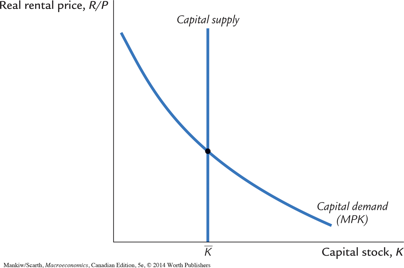
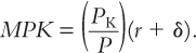
Let’s first consider the typical production firm. As we discussed in Chapter 3, this firm decides how much capital to rent by comparing the cost and benefit of each unit of capital. The firm rents capital at a rental rate R and sells its output at a price P; the real cost of a unit of capital to the production firm is R/P. The real benefit of a unit of capital is the marginal product of capital MPK—the extra output produced with one more unit of capital. The marginal product of capital declines as the amount of capital rises: the more capital the firm has, the less an additional unit of capital will add to its output. Chapter 3 concluded that, to maximize profit, the firm rents capital until the marginal product of capital falls to equal the real rental price.
Figure 18-2 shows the equilibrium in the rental market for capital. For the reasons just discussed, the marginal product of capital determines the demand curve. The demand curve slopes downward because the marginal product of capital is low when the level of capital is high. At any point in time, the amount of capital in the economy is fixed, so the supply curve is vertical. The real rental price of capital adjusts to equilibrate supply and demand.
608
To see what variables influence the equilibrium rental price, let’s consider a particular production function. As we saw in Chapter 3, many economists consider the Cobb–Douglas production function a good approximation of how the actual economy turns capital and labour into goods and services. The Cobb–Douglas production function is
Y = AKαL1–α,
where Y is output, K capital, L labour, A a parameter measuring the level of technology, and α a parameter between zero and one that measures capital’s share of output. The marginal product of capital for the Cobb–Douglas production function is
MPK = αA(L/K)1–α.
Because the real rental price equals the marginal product of capital in equilibrium, we can write
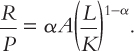
This expression identifies the variables that determine the real rental price. It shows the following:
The lower the stock of capital, the higher the real rental price of capital
The greater the amount of labour employed, the higher the real rental price of capital
The better the technology, the higher the real rental price of capital
Events that reduce the capital stock (an earthquake), or raise employment (an expansion in aggregate demand), or improve the technology (a scientific discovery) raise the equilibrium real rental price of capital.
The Cost of Capital
Next consider the rental firms. These firms, like car-rental companies, merely buy capital goods and rent them out. Since our goal is to explain the investments made by the rental firms, we begin by considering the benefit and cost of owning capital.
The benefit of owning capital is the revenue earned by renting it to the production firms. The rental firm receives the real rental price of capital R/P for each unit of capital it owns and rents out.
The cost of owning capital is more complex. For each period of time that it rents out a unit of capital, the rental firm bears three costs:
When a rental firm borrows to buy a unit of capital, which it intends to rent out, it must pay interest on the loan. If PK is the purchase price of a unit of capital and i is the nominal interest rate, then iPK is the interest cost. Notice that this interest cost would be the same even if the rental firm did not have to borrow: if the rental firm buys a unit of capital using cash on hand, it loses out on the interest it could have earned by depositing this cash in the bank. In either case, the interest cost equals iPK.
609
While the rental firm is renting out the capital, the price of capital can change. If the price of capital falls, the firm loses, because the firm’s asset has fallen in value. If the price of capital rises, the firm gains, because the firm’s asset has risen in value. The cost of this loss or gain is –Δ PK. (The minus sign is here because we are measuring costs, not benefits.)
While the capital is rented out, it suffers wear and tear, called depreciation. If δ is the rate of depreciation—the fraction of value lost per period because of wear and tear—then the dollar cost of depreciation is δPK.
The total cost of renting out a unit of capital for one period is therefore
Cost of Capital = iPK – ΔPK + δPK
= PK(i– ΔPK/PK + δ).
The cost of capital depends on the price of capital, the interest rate, the rate at which capital prices are changing, and the depreciation rate.
For example, consider the cost of capital to a car-rental company. The company buys cars for $10,000 each and rents them out to other businesses. The company faces an interest rate i of 10 percent per year, so the interest cost iPK is $1,000 per year for each car the company owns. Car prices are rising at 6 percent per year, so, excluding wear and tear, the firm gets a capital gain ΔPK of $600 per year. Cars depreciate at 20 percent per year, so the loss due to wear and tear δPK is $2,000 per year. Therefore, the company’s cost of capital is
Cost of Capital = $1,000 – $600 + $2,000
= $2,400.
The cost to the car-rental company of keeping a car in its capital stock is $2,400 per year.
To make the expression for the cost of capital simpler and easier to interpret, we assume that the price of capital goods rises with the prices of other goods. In this case, ΔPK/PK equals the overall rate of inflation π. Because i – π equals the real interest rate r, we can write the cost of capital as
Cost of Capital = PK(r + δ).
This equation states that the cost of capital depends on the price of capital, the real interest rate, and the depreciation rate.
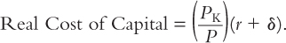
Finally, we want to express the cost of capital relative to other goods in the economy. The real cost of capital—the cost of buying and renting out a unit of capital measured in units of the economy’s output—is
610
This equation states that the real cost of capital depends on the relative price of a capital good PK/P, the real interest rate r, and the depreciation rate δ.
The Determinants of Investment
Now consider a rental firm’s decision about whether to increase or decrease its capital stock. For each unit of capital, the firm earns real revenue R/P and bears the real cost (PK/P)(r + δ). The real profit per unit of capital is
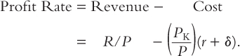
Because the real rental price in equilibrium equals the marginal product of capital, we can write the profit rate as
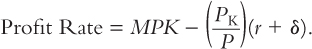
The rental firm makes a profit if the marginal product of capital is greater than the cost of capital. It incurs a loss if the marginal product is less than the cost of capital.
We can now see the economic incentives that lie behind the rental firm’s investment decision. The firm’s decision regarding its capital stock—that is, whether to add to it or to let it depreciate—depends on whether owning and renting out capital is profitable. The change in the capital stock, called net investment, depends on the difference between the marginal product of capital and the cost of capital. If the marginal product of capital exceeds the cost of capital, firms find it profitable to add to their capital stock. If the marginal product of capital falls short of the cost of capital, they let their capital stock shrink.
We can also now see that the separation of economic activity between production and rental firms, although useful for clarifying our thinking, is not necessary for our conclusion regarding how firms choose how much to invest. For a firm that both uses and owns capital, the benefit of an extra unit of capital is the marginal product of capital, and the cost is the cost of capital. Like a firm that owns and rents out capital, this firm adds to its capital stock if the marginal product exceeds the cost of capital. Thus, we can write
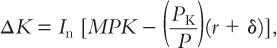
where In[ ] is the function showing how much net investment responds to the incentive to invest.
We can now derive the investment function. Total spending on business fixed investment is the sum of net investment and the replacement of depreciated capital. The investment function is
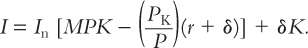
Business fixed investment depends on the marginal product of capital, the cost of capital, and the amount of depreciation.
611
This model shows why investment depends on the interest rate. A decrease in the real interest rate lowers the cost of capital. It therefore raises the amount of profit from owning capital and increases the incentive to accumulate more capital. Similarly, an increase in the real interest rate raises the cost of capital and leads firms to reduce their investment. For this reason, the investment schedule relating investment to the interest rate slopes downward, as in panel (a) of Figure 18-3.
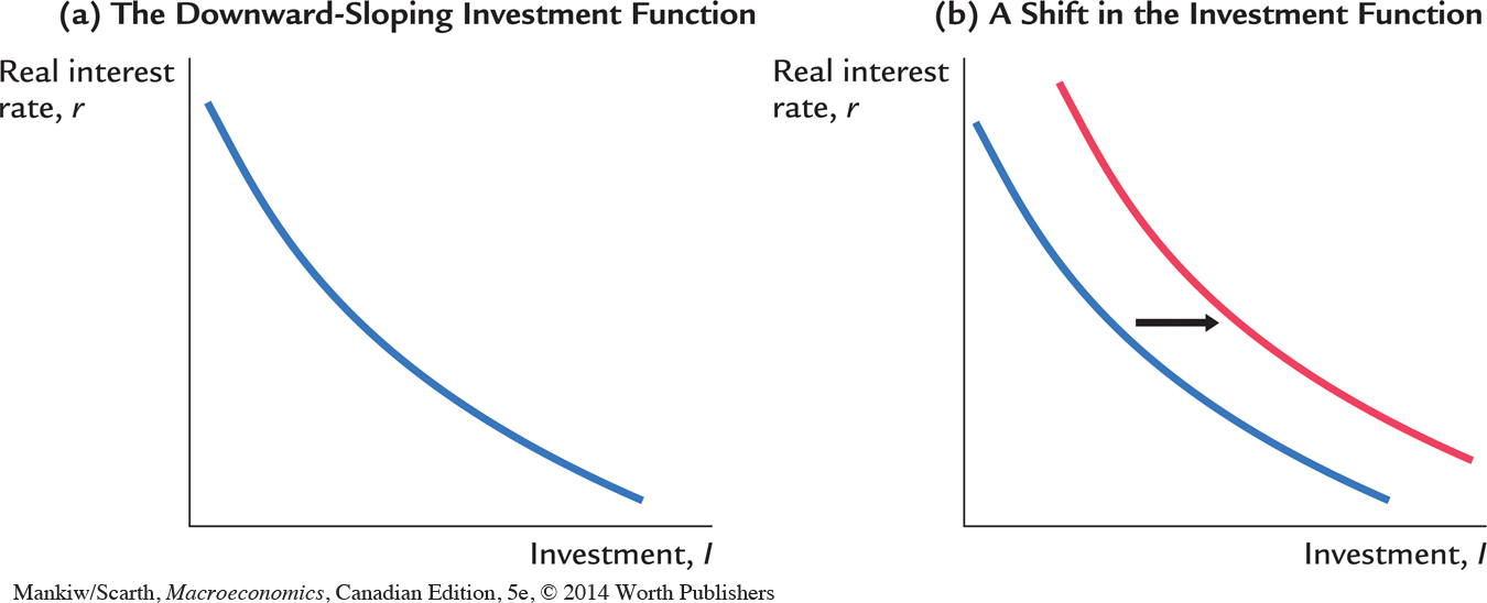
The model also shows what causes the investment schedule to shift. Any event that raises what business managers expect the marginal product of capital to be, increases the profitability of investment and causes the investment schedule to shift outward, as in panel (b) of Figure 18-3. For example, a technological innovation that increases the production function parameter A raises the marginal product of capital and, for any given interest rate, increases the amount of capital goods that rental firms wish to buy. Similarly, a drop on consumer confidence will lead managers to fear that their sales will be low. In revenue terms, then capital’s marginal product is expected to be low, so the investment schedule shifts inward.
Finally, consider what happens as this adjustment of the capital stock continues over time. If the marginal product begins above the cost of capital, the capital stock will rise and the marginal product will fall. If the marginal product of capital begins below the cost of capital, the capital stock will fall and the marginal product will rise. Eventually, as the capital stock adjusts, the marginal product of capital approaches the cost of capital. When the capital stock reaches a steady-state level, we can write
612
Thus, in the long run, the marginal product of capital equals the real cost of capital. The speed of adjustment toward the steady state depends on how quickly firms adjust their capital stock, which in turn depends on how costly it is to build, deliver, and install new capital.1
CASE STUDY
The Burden of Higher Interest Rates
Journalists frequently refer to high interest rates as a “burden” for Canadians. There are two reasons for this, and we are now in a position to appreciate this concern. First, in the short run, an increase in interest rates pulls investment down and so lowers aggregate demand. With prices sticky in the short run, a recession can result. But this line of argument cannot explain why a one-time, but permanent, rise in interest rates is a burden. After all, investment will not keep falling—long after the one-time increase in borrowing costs—and with flexible prices in the long run, real GDP should gradually return to its natural level.
But that natural level will be lower since it involves a smaller capital stock; as we have learned, firms arrange their affairs so that the marginal product of capital equals the real (rental) cost of capital:
MPK = r + δ.
(Units have been chosen so that the purchase price of capital, PK, equals the purchase price of other goods, P.) In Chapter 3, we learned that the Cobb–Douglas production function is a good approximation of production processes in Canada, and that for this production function, the marginal product of capital is given by
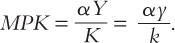
where α is capital’s share of output. Substituting this expression for MPK into the steady-state capital-demand relationship yields
αy = (r + δ)k.
Rewriting this equilibrium condition in change form (holding α and δ constant) results in
αΔy = (r + δ)Δk + kΔr.
613
Since we also know that Δy = MPKΔk = (r + δ)Δk, we can use this relationship to eliminate Δk by substitution. The result, after dividing by y, is
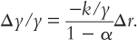
We can use this equation to illustrate the steady-state “burden” of higher interest rates. Suppose the real interest rate increases permanently by one-half of one percentage point. To see the implications, we substitute Δr =Δ0.005 into the equation, along with representative values for the other parameters, (k/y) = 3 and α = 0.33. The result is
Δy/y = – 2.2 percent.
This result implies that Canadians lose an amount of material welfare equal to 2.2 percent of GDP every year if the interest rate is permanently higher by just one half of one percentage point. As this book goes to press, this loss amounts to $35 billion every year. This annual loss represents a lot of valuable items, such as hospitals and day-care facilities. It appears that standard macroeconomic analysis supports journalists who refer to even “small” increases in interest rates as a major “burden.” 
Taxes and Investment
Tax laws influence firms’ incentives to accumulate capital in many ways. Sometimes policymakers change the tax laws in order to shift the investment function and influence aggregate demand. Here we consider three of the most important provisions of corporate taxation: the corporate profit tax rate itself, depreciation allowances, and the investment tax credit.
The effect of a corporate profit tax on investment depends on how the law defines “profit” for the purpose of taxation. Suppose, first, that the law defined profit as we did above—the rental price of capital minus the cost of capital. In this case, even though firms would be sharing a fraction of their profits with the government, it would still be rational for them to invest if the rental price of capital exceeded the cost of capital, and to disinvest if the rental price fell short of the cost of capital. A tax on profit, measured in this way, would not alter investment incentives.
Yet, because of the tax law’s definition of profit, the corporate profit tax does affect investment decisions. There are many differences between the law’s definition of profit and ours. One major difference is the treatment of depreciation. Our definition of profit deducts the current value of depreciation as a cost. That is, it bases depreciation on how much it would cost today to replace worn-out capital. By contrast, under the corporate tax laws, firms deduct depreciation using historical cost. That is, the depreciation allowance is based on the price of the capital when it was originally purchased. In periods of inflation, true replacement cost is greater than historical cost, so the corporate tax tends to understate the cost of depreciation and overstate profit. As a result, the tax law sees a profit and levies a tax even when economic profit is zero, which makes owning capital less attractive. For this and other reasons, many economists believe that the corporate profit tax discourages investment.
The investment tax credit is a tax provision that encourages the accumulation of capital. The investment tax credit reduces a firm’s taxes by a certain amount for each dollar spent on capital goods. Because a firm recoups part of its expenditure on new capital in lower taxes, the credit reduces the effective purchase price of a unit of capital PK. Thus, the investment tax credit reduces the cost of capital and raises investment.
614
Tax incentives for investment are one tool policymakers can use to control aggregate demand. For example, an increase in the investment tax credit reduces the cost of capital, shifts the investment function outward, and raises aggregate demand. Similarly, a reduction in the tax credit reduces aggregate demand by making investment more costly.
From the mid-1950s to the mid-1970s, the government of Sweden attempted to control aggregate demand by encouraging or discouraging investment. A system called the investment fund subsidized investment, much like an investment tax credit, during periods of recession. When government officials decided that economic growth had slowed, they authorized a temporary investment subsidy. When the officials concluded that the economy had recovered sufficiently, they revoked the subsidy. Eventually, however, Sweden abandoned the use of temporary investment subsidies to control the business cycle, and the subsidy became a permanent feature of Swedish tax policy.
Should investment subsidies be used to combat economic fluctuations? Some economists believe that for the two decades it was in effect the Swedish policy reduced the magnitude of the business cycle. Others believe that such a policy could have had unintended and perverse effects: for example, if the economy begins to slow down, firms may anticipate a future subsidy and delay investment, making the slowdown worse. Because the use of countercyclical investment subsidies could either reduce or amplify the size of economic fluctuations, their overall impact on economic performance is hard to evaluate.2
CASE STUDY
Canada’s Experience with Corporate Tax Concessions
Capital goods typically wear out at a slower rate than that assumed by the tax laws. Firms would like governments to think that all capital goods completely wear out during the purchase year, so that they can claim the entire cost of the machine as a current expense. By reducing reported profits that first year, tax obligations are less. Of course in later years, because firms have already claimed the full expense for the machine, reported profits (and therefore tax obligations) are then larger. But a tax saving today is worth more than one in the future, and firms are happy to accept an interest-free loan from governments whenever they can.
615
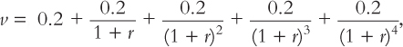
The corporate tax laws define how rapidly machinery wears out for tax purposes. For example, in the manufacturing and processing sector, depreciation allowances have allowed one-half the machinery expense to be claimed in each of the first two years following its purchase. As far as generating a tax deduction, the present value of each dollar spent on investment is
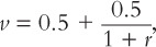
where r is the rate of interest. With an interest rate of 8 percent, for example, this formula implies that v is 0.963.
The Canadian legislation is almost as generous as the tax law can be. The maximum possible value for v is 1, and this occurs if firms are allowed to claim the entire cost of the machinery in the first year. A less generous depreciation allowance makes v lower. For example, if, for tax purposes, machinery is deemed to wear out over five years, the formula for v is
and, for the assumed 8 percent interest rate, v is 0.86. The federal government has opted for generous depreciation allowances in an attempt to stimulate investment expenditures.
Another initiative of the government is to reduce the corporate income tax rate itself. But this policy has often proven to be a very inefficient way to stimulate investment spending. We can understand why by noting that a lower tax rate brings both a benefit and a cost to firms. If it were not for the allowed deductions for depreciation, a 10-percent cut in the corporate tax rate would lower tax obligations by 10 percent. But a lower tax rate means that smaller deductions can be claimed. The loss in deduction equals v times 10 percent.
With v almost unity in Canada, it makes almost no sense to cut the corporate tax rate. The benefit and the cost to firms change by almost the same amount, so the incentive for firms to invest is hardly increased at all—despite a major revenue loss for the government. Thus introducing accelerated depreciation allowances (raising v) can stimulate investment spending, but once this has been done, the rationale for cutting the tax rate itself is reduced.
This discussion pertains to Canadian-owned firms. The case against using corporate tax concessions as a means of stimulating investment spending is even stronger in the case of foreign-owned firms. Firms that are subsidiaries of multinationals based in other countries get to deduct all taxes paid in Canada when calculating corporate taxes in their home countries (up to an amount equal to what they would have paid in their home country). In this case, the corporate tax concession in Canada does not lower the rental cost of capital. These tax concessions simply transfer revenue to foreign governments, and so they have no effect on investment.
The Stock Market and Tobin’s q
616
Many economists see a link between fluctuations in investment and fluctuations in the stock market. The term stock refers to the shares in the ownership of corporations, and the stock market is the market in which these shares are traded. Stock prices tend to be high when firms have many opportunities for profitable investment, since these profit opportunities mean higher future income for the shareholders. Thus, stock prices reflect the incentives to invest.
The Nobel-Prize-winning economist James Tobin proposed that firms base their investment decisions on the following ratio, which is now called Tobin’s q:
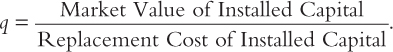
The numerator of Tobin’s q is the value of the economy’s capital as determined by the stock market. The denominator is the price of the capital if it were purchased today.
Tobin reasoned that net investment should depend on whether q is greater or less than 1. If q is greater than 1, then the stock market values installed capital at more than its replacement cost. In this case, managers can raise the market value of their firms’ stock by buying more capital. Conversely, if q is less than 1, the stock market values capital at less than its replacement cost. In this case, managers will not replace capital as it wears out.
Although at first the q theory of investment may appear quite different from the neoclassical model developed above, in fact the two theories are closely related. To see the relationship, note that Tobin’s q depends on current and future expected profits from installed capital. If the marginal product of capital exceeds the cost of capital, then firms are earning profit on their installed capital. These profits make the rental firms desirable to own, which raises the market value of these firms’ stock, implying a high value of q. Similarly, if the marginal product of capital falls short of the cost of capital, then firms are incurring losses on their installed capital, implying a low market value and a low value of q.
Formally, the q theory and the neoclassical model can be related as follows. The owners of capital receive the MPK for each unit of capital every year forever. Assuming, for simplicity, that capital’s marginal product is expected to stay constant in the future, the present value of that stream of receipts in nominal terms is
P(MPK)(x + x2 + . . .),
where
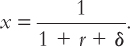
617
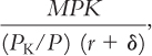
Since (x + x2 + ...) equals [(1 + x + x2 + ...) – 1], and since we learned in Chapter 10 that the geometric series (1 + x + x2 + . . .) equals [(1/1 – x)], we can simplify the present value of receipts expression to

for each unit of capital. The discount factor, (r + δ), involves the rate at which interest is forgone by tying up funds in the ownership of capital, r, and the rate at which capital is wearing out, δ Buyers and sellers in the stock market should recognize that this present value is what an owner of the stock receives. Thus, this present value, when multiplied by the total quantity of capital, is the market value of the existing capital stock. q is the ratio of this market value to the purchase cost of capital PKK. Thus, q is
and q > 1 implies that capital’s marginal product exceeds its rental cost, so investment is profitable.
Finally, the investment function can be derived more formally by specifying that firms minimize the following cost function:
(Kt – Kt*)2 + θ(Kt – Kt–1)2,
where K and K* denote the actual and desired levels of the capital stock and the subscripts indicate time periods. Firms incur costs when the capital stock is not at its desired value (when K differs from K*), and they incur disruption costs whenever they adjust their holdings of capital (when the current value of K differs from its value in the previous time period). The two terms in the cost function capture these two considerations. The quadratic form is the simplest function that does so, and parameter θ represents the relative importance of the adjustment costs.
With both the long-run desired level of capital and the preexisting level of capital given at each point in time, firms minimize costs by differentiating the cost function with respect to Kt and setting the result equal to zero. The result is
(Kt – Kt-1) = γ (Kt* – Kt–1)
where γ = 1/(1 + θ), or more simply,
ΔK = γ (K* – K)
or
ΔK/K = γ [(K*/K) – 1].
Since γ is a fraction, this investment function involves net investment closing a fraction of the gap between the desired and the actual capital stock each period. And we have just learned that the (K*/K) ratio exceeds unity whenever the rental price of capital exceeds the cost of capital—that is, when Tobin’s q exceeds one.
The advantage of Tobin’s q as a measure of the incentive to invest is that it reflects the expected future profitability of capital as well as the current profitability. For example, suppose that the federal government legislates a reduction in the corporate profit tax beginning next year. This expected fall in the corporate tax means greater profits for the owners of capital. These higher expected profits raise the value of stock today, raise Tobin’s q, and therefore encourage investment today. Thus, Tobin’s q theory of investment emphasizes that investment decisions depend not only on current economic policies, but also on policies expected to prevail in the future.3
618
Keynes argued that firm managers and households that buy the firm’s stocks have quite volatile expectations. This fact is reflected in Tobin’s q rising and falling fairly dramatically over time. According to the theory, investment spending should be a very volatile component of aggregate demand—and it is. Keynes emphasized this fact by arguing that investment is as much a function of people’s waves of optimism and pessimism (what he called their “animal spirits”) as it is a function of the interest rate. It is reassuring that, according to the q theory, both are important influences on investment.
CASE STUDY
The Stock Market as an Economic Indicator
“The stock market has predicted nine out of the last five recessions.” So goes Paul Samuelson’s famous quip about the stock market’s reliability as an economic indicator. The stock market is in fact quite volatile, and it can give false signals about the future of the economy. Yet one should not ignore the link between the stock market and the economy. Figure 18-4 shows that changes in the stock market often reflect changes in real GDP.
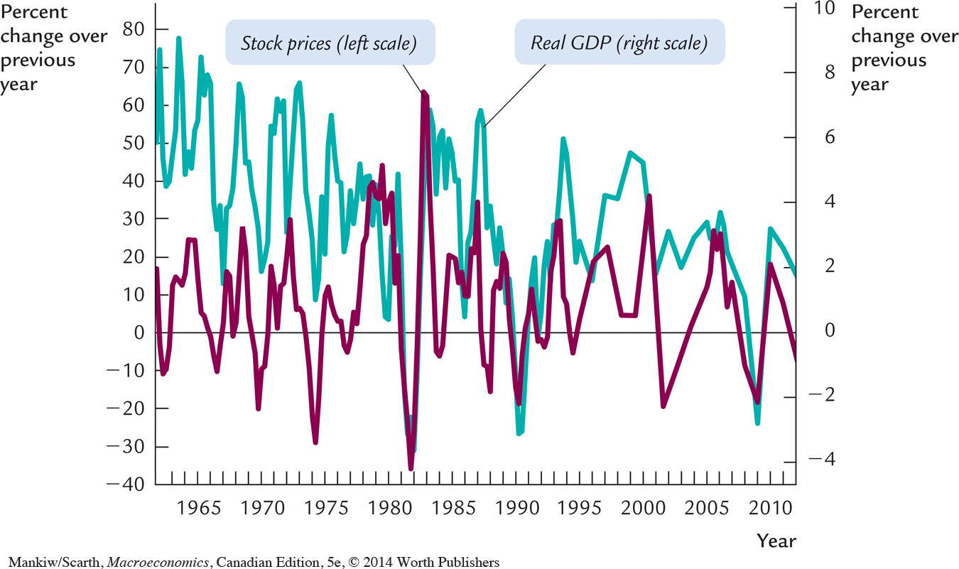
Why do stock prices and economic activity tend to fluctuate together? One reason is given by Tobin’s q theory, together with the model of aggregate demand and aggregate supply. Suppose, for instance, that you observe a fall in stock prices. Because the replacement cost of capital is fairly stable, a fall in the stock market is usually associated with a fall in Tobin’s q. A fall in q reflects investors’ pessimism about the current or future profitability of capital. This means that the investment function has shifted inward: investment is lower at any given interest rate. As a result, the aggregate demand for goods and services contracts, leading to lower output and employment.
There are two additional reasons why stock prices are associated with economic activity. First, because stock is part of household wealth, a fall in stock prices makes people poorer and thus depresses consumer spending, which also reduces aggregate demand. Second, a fall in stock prices might reflect bad news about technological progress and long-run economic growth. If so, this means that the natural level of output—and thus aggregate supply—will be growing more slowly in the future than was previously expected.
619
These links between the stock market and the economy are not lost on policymakers, such as those at the Bank of Canada. Indeed, because the stock market often anticipates changes in real GDP, and because data on the stock market are available more quickly than data on GDP, the stock market is a closely watched economic indicator. A case in point is the economic downturn in 2009; the substantial decline in production and employment was preceded by a steep decline in stock prices.
Alternative Views of the Stock Market: The Efficient Markets Hypothesis Versus Keynes’s Beauty Contest
One continuing source of debate among economists is whether stock market fluctuations are rational.
Some economists subscribe to the efficient markets hypothesis, according to which the market price of a company’s stock is the fully rational valuation of the company’s value, given current information about the company’s business prospects. This hypothesis rests on two foundations:
620
Each company listed on a major stock exchange is followed closely by many professional portfolio managers, such as the individuals who run mutual funds. Every day, these managers monitor news stories to try to determine the company’s value. Their job is to buy a stock when its price falls below its value and to sell it when its price rises above its value.
The price of each stock is set by the equilibrium of supply and demand. At the market price, the number of shares being offered for sale exactly equals the number of shares that people want to buy. That is, at the market price, the number of people who think the stock is overvalued exactly balances the number of people who think it’s undervalued. As judged by the typical person in the market, the stock must be fairly valued.
According to this theory, the stock market is informationally efficient: it reflects all available information about the value of the asset. Stock prices change when information changes. When good news about the company’s prospects becomes public, the value and the stock price both rise. When the company’s prospects deteriorate, the value and price both fall. But at any moment in time, the market price is the rational best guess of the company’s value based on available information.
One implication of the efficient markets hypothesis is that stock prices should follow a random walk. This means that the changes in stock prices should be impossible to predict from available information. If, based on publicly available information, a person could predict that a stock price would rise by 10 percent tomorrow, then the stock market must be failing to incorporate that information today. According to this theory, the only thing that can move stock prices is news that changes the market’s perception of the company’s value. But such news must be unpredictable—otherwise, it wouldn’t really be news. For the same reason, changes in stock prices should be unpredictable as well.
What is the evidence for the efficient markets hypothesis? Its proponents point out that it is hard to beat the market by buying allegedly undervalued stocks and selling allegedly overvalued stocks. Statistical tests show that stock prices are random walks, or at least approximately so. Moreover, index funds, which buy stocks from all companies in a stock market index, outperform most actively managed mutual funds run by professional money managers.
Although the efficient markets hypothesis has many proponents, some economists are less convinced that the stock market is so rational. These economists point out that many movements in stock prices are hard to attribute to news. They suggest that, when buying and selling, stock investors are less focused on companies’ fundamental values than on what they expect other investors will later pay.
John Maynard Keynes proposed a famous analogy to explain stock market speculation. In his day, some newspapers held beauty contests in which the paper printed the picture of 100 women and readers were invited to submit a list of the five most beautiful. A prize went to the reader whose choices most closely matched those of the consensus of the other entrants. A naïve entrant would have simply picked the five most beautiful women. But a slightly more sophisticated strategy would have been to guess the five women that other people considered the most beautiful. Other people, however, were likely thinking along the same lines. So an even more sophisticated strategy would have been to try to guess what other people thought other people thought were the most beautiful women. And so on. In the end of the process, judging true beauty would be less important to winning the contest than guessing other people’s opinions of other people’s opinions.
621
Similarly, Keynes reasoned that, because stock market investors will eventually sell their shares to others, they were more concerned about other people’s valuation of a company than the company’s true worth. The best stock investors, in his view, were those who were good at outguessing mass psychology. He believed that movements in stock prices often reflect irrational waves of optimism and pessimism (the “animal spirits”) of investors.
The two views of the stock market persist to this day. Some economists see the stock market through the lens of the efficient markets hypothesis. They believe fluctuations in stock prices are a rational reflection of changes in under-lying economic fundamentals. Other economists, however, take Keynes’s beauty contest as a metaphor for stock speculation. In their view, the stock market often fluctuates for no good reason, and because it influences the aggregate demand for goods and services, these fluctuations are a source of short-run economic fluctuations.4
Financing Constraints
When a firm wants to invest in new capital, say by building a new factory, it often raises the necessary funds in financial markets. This financing may take several forms: obtaining loans from banks, selling bonds to the public, or selling shares in future profits on the stock market. The neoclassical model assumes that if a firm is willing to pay the cost of capital, the financial markets will make the funds available.
Yet sometimes firms face financing constraints—limits on the amount they can raise in financial markets. Financing constraints can prevent firms from undertaking profitable investments. When a firm is unable to raise funds in financial markets, the amount it can spend on new capital goods is limited to the amount it is currently earning. Financing constraints influence the investment behaviour of firms just as borrowing constraints influence the consumption behaviour of households. Borrowing constraints cause households to determine their consumption on the basis of current rather than permanent income; financing constraints cause firms to determine their investment on the basis of their current cash flow rather than expected profitability.
622
To see the impact of financing constraints, consider the effect of a short recession on investment spending. A recession reduces employment, the rental price of capital, and profits. If firms expect the recession to be short-lived, however, they will want to continue investing, knowing that their investments will be profitable in the future. That is, a short recession will have only a small effect on Tobin’s q. For firms that can raise funds in financial markets, the recession should have only a small effect on investment.
Quite the opposite is true for firms that face financing constraints. The fall in current profits restricts the amount that these firms can spend on new capital goods and may prevent them from making profitable investments. Thus, financing constraints make investment more sensitive to current economic conditions.5
Banking Crises and Credit Crunches
Throughout economic history, problems in the banking system have often co-incided with downturns in economic activity. This was true, for instance, during the Great Depression of the 1930s (which we discussed in Chapter 11). Soon after the Depression’s onset, many banks in the United States found themselves insolvent, as the value of their assets fell below the value of their liabilities. These banks were, therefore, forced to suspend operations. Many economists believe the widespread bank failures in the United States during this period help explain the Depression’s depth and persistence.
Similar patterns, although less severe, can be observed more recently. Problems in the banking system were also part of a slump in Japan and of the financial crises in Indonesia and other Asian economies (as we saw in Chapter 12). More recently, in the United States, the recession of 2008–2009 came on the heels of a widespread financial crisis that began with a downturn in the housing market (as we discussed in Chapter 11).
Why are banking crises so often at the center of economic downturns? Banks have an important role in the economy because they allocate financial resources to their most productive uses: they serve as intermediaries between those people who have income they want to save and those people who have profitable investment projects but need to borrow the funds to invest. When banks become insolvent or nearly so, they are less able to serve this function. Financing constraints become more prevalent, and some investors are forced to forgo some potentially profitable investment projects. Such an increase in financing constraints is sometimes called a credit crunch.
623
We can use the IS–LM model to interpret the short-run effects of a credit crunch. When some would-be investors are denied credit, the demand for investment goods falls at every interest rate. The result is a contractionary shift in the IS curve, which in turn leads to a fall in aggregate demand and reduced production and employment. The long-run effects of a credit crunch are best understood from the perspective of growth theory, with its emphasis on capital accumulation as a source of growth. When a credit crunch prevents some firms from investing, the financial markets fail to allocate national saving to its best use. Less productive investment projects may take the place of more productive projects, reducing the economy’s potential for producing goods and services.
Because of these effects, central bankers are always trying to monitor the health of the nation’s banking system. Their goal is to avert banking crises and credit crunches and, when they do occur, to respond as quickly as possible to minimize the resulting disruption to the economy. That job is not easy, as the financial crisis and economic downturn of 2008–2009 illustrates. In this case, as we discussed in Chapter 11, many banks had made large bets on the housing markets through their purchases of mortgage-backed securities. When those bets turned bad, many banks found themselves insolvent or nearly so, and bank loans became hard to come by. Bank regulators at the Federal Reserve and other U.S. government agencies, like many of the bankers themselves, were caught off guard by the magnitude of the losses and the resulting precariousness of the banking system. What kind of regulatory changes will be needed to try to reduce of likelihood of future banking crises remains a topic of active debate.