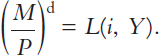
We now turn to the other side of the money market and examine what determines money demand. In previous chapters, we used simple money demand functions. We started with the quantity theory, which assumes that the demand for real balances is proportional to income. That is, the quantity theory assumes

646

(M/P)^d = kY,

where k is a constant measuring how much money people want to hold for every dollar of income. We then considered a more general and realistic money demand function that assumes the demand for real money balances depends on both the interest rate and income:

We used this money demand function when we discussed the link between money and prices in Chapter 4 and when we developed the IS–LM model in Chapters 10 and 11.

There is, of course, much more to say about what determines how much money people choose to hold. Just as studies of the consumption function rely on microeconomic models of the consumption decision, studies of the money demand function rely on microeconomic models of the money demand decision. In this section we first discuss in broad terms the different ways to model money demand. We then develop one prominent model.

Recall that money serves three functions: it is a unit of account, a store of value, and a medium of exchange. The first function—money as a unit of account—does not by itself generate any demand for money, because one can quote prices in dollars without holding any. By contrast, money can serve its other two functions only if people hold it. Theories of money demand emphasize the role of money either as a store of value or as a medium of exchange.

Theories of money demand that emphasize the role of money as a store of value are called portfolio theories. According to these theories, people hold money as part of their portfolio of assets. The key insight is that money offers a different combination of risk and return than other assets. In particular, money offers a safe (nominal) return, whereas the prices of stocks and bonds may rise or fall. Thus, some economists have suggested that households choose to hold money as part of their optimal portfolio.²

Portfolio theories predict that the demand for money should depend on the risk and return offered by money and by the various assets households can hold instead of money. In addition, money demand should depend on total wealth, because wealth measures the size of the portfolio to be allocated among money and the alternative assets. For example, we might write the money demand function as

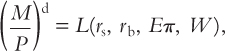
where r_s is the expected real return on stock, r_b is the expected real return on bonds, Eπ is the expected inflation rate, and W is real wealth. An increase in r_s or r_b reduces money demand, because other assets become more attractive. An increase in Eπ also reduces money demand, because money becomes less attractive. (Recall that – Eπ is the expected real return to holding money.) An increase in W raises money demand, because higher wealth means a larger portfolio.

647

From the standpoint of portfolio theories, we can view our money demand function, L(i, Y), as a useful simplification. First, it uses real income Y as a proxy for real wealth W. If we think of wealth very broadly defined to include human capital, income is the yield on wealth. Second, the only return variable it includes is the nominal interest rate, which is the sum of the real return on bonds and expected inflation (that is, i = r_b + Eπ). According to portfolio theories, however, the money demand function should include the expected returns on other assets as well.

Are portfolio theories useful for studying money demand? The answer depends on which measure of money we are considering. The most narrow measures of money, such as M1, include only currency and deposits in chequing accounts. These forms of money earn zero or very low rates of interest. There are other assets—such as savings accounts, treasury bills, and guaranteed investment certificates—that earn higher rates of interest and have the same risk characteristics as currency and chequing accounts. Economists say that money (M1) is a dominated asset: as a store of value, it exists alongside other assets that are always better. Thus, it is not optimal for people to hold money as part of their portfolio, and portfolio theories cannot explain the demand for these dominated forms of money.

Portfolio theories are more plausible as theories of money demand if we adopt a broad measure of money. The broad measures include many of those assets that dominate currency and chequing accounts. M2, for example, includes savings and other notice accounts. When we examine why people hold assets in the form of M2, rather than bonds or stock, the portfolio considerations of risk and return may be paramount. Hence, although the portfolio approach to money demand may not be plausible when applied to M1, it may be a good theory to explain the demand for M2 or M3.

Theories of money demand that emphasize the role of money as a medium of exchange are called transactions theories. These theories acknowledge that money is a dominated asset and stress that people hold money, unlike other assets, to make purchases. These theories best explain why people hold narrow measures of money, such as currency and chequing accounts, as opposed to holding assets that dominate them, such as savings accounts or treasury bills.

Transactions theories of money demand take many forms, depending on how one models the process of obtaining money and making transactions. All these theories assume that money has the cost of earning a low rate of return and the benefit of making transactions more convenient. People decide how much money to hold by trading off these costs and benefits.

To see how transactions theories explain the money demand function, let’s develop one prominent model of this type. The Baumol–Tobin model was developed in the 1950s by economists William Baumol and James Tobin, and it remains a leading theory of money demand.³

The Baumol–Tobin model analyzes the costs and benefits of holding money. The benefit of holding money is convenience: people hold money to avoid making a trip to the bank every time they wish to buy something. The cost of this convenience is the forgone interest they would have received had they left the money deposited in a savings account that paid interest.

To see how people trade off these benefits and costs, consider a person who plans to spend Y dollars gradually over the course of a year. (For simplicity, assume that the price level is constant, so real spending is constant over the year.) How much money should he hold in the process of spending this amount? That is, what is the optimal size of average cash balances?

649

Consider the possibilities. He could withdraw the Y dollars at the beginning of the year and gradually spend the money. Panel (a) of Figure 19-1 shows his money holdings over the course of the year under this plan. His money holdings begin the year at Y and end the year at zero, averaging Y/2 over the year.

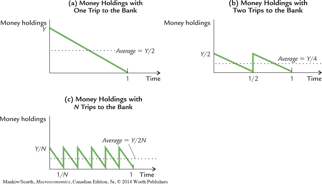
A second possible plan is to make two trips to the bank. In this case, he withdraws Y/2 dollars at the beginning of the year, gradually spends this amount over the first half of the year, and then makes another trip to withdraw Y/2 for the second half of the year. Panel (b) of Figure 19-1 shows that money holdings over the year vary between Y/2 and zero, averaging Y/4. This plan has the advantage that less money is held on average, so the individual forgoes less interest, but it has the disadvantage of requiring two trips to the bank rather than one.

More generally, suppose the individual makes N trips to the bank over the course of the year. On each trip, he withdraws Y/N dollars; he then spends the money gradually over the following 1/Nth of the year. Panel (c) of Figure 19-1 shows that money holdings vary between Y/N and zero, averaging Y/(2N).

The question is, what is the optimal choice of N? The greater N is, the less money the individual holds on average and the less interest he forgoes. But as N increases, so does the inconvenience of making frequent trips to the bank.

Suppose that the cost of going to the bank is some fixed amount F. We can view F as representing the value of the time spent traveling to and from the bank and waiting in line to make the withdrawal. For example, if a trip to the bank takes 15 minutes and a person’s wage is $12 per hour, then F is $3. Also, let i denote the interest rate; because money does not bear interest, i measures the opportunity cost of holding money.

650

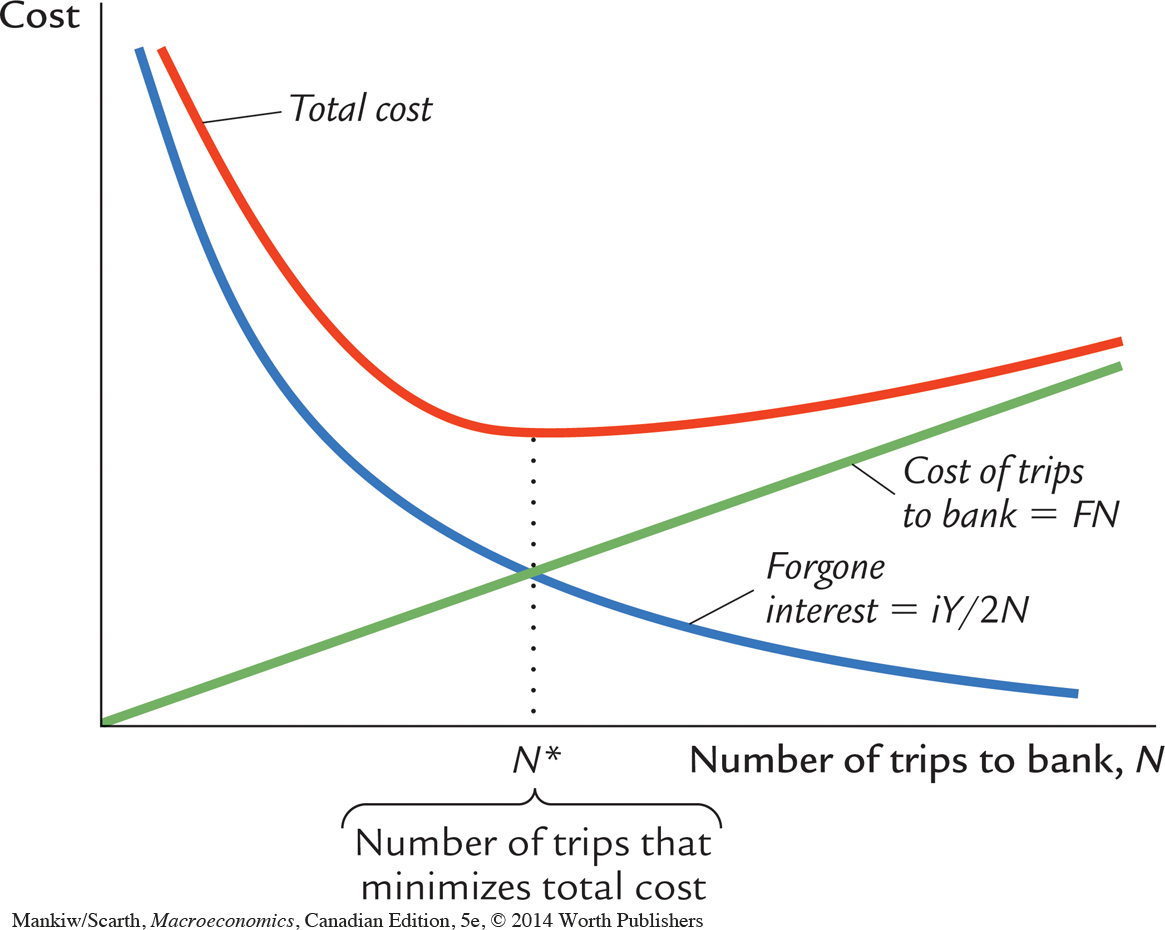
Now we can analyze the optimal choice of N, which determines money demand. For any N, the average amount of money held is Y/(2N), so the forgone interest is iY/(2N). Because F is the cost per trip to the bank, the total cost of making trips to the bank is FN. The total cost the individual bears is the sum of the forgone interest and the cost of trips to the bank:

Total Cost = Forgone Interest + Cost of Trips

= iY/(2N) + FN.

The larger the number of trips N, the smaller the forgone interest, and the larger the cost of going to the bank.

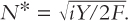
Figure 19-2 shows how total cost depends on N. There is one value of N that minimizes total cost. The optimal value of N, denoted N*, is⁴

651

Average money holding is

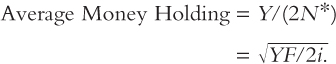
This expression shows that the individual holds more money if the fixed cost of going to the bank F is higher, if expenditure Y is higher, or if the interest rate i is lower.

So far, we have been interpreting the Baumol–Tobin model as a model of the demand for currency. That is, we have used it to explain the amount of money held outside of banks. Yet one can interpret the model more broadly. Imagine a person who holds a portfolio of monetary assets (currency and chequing accounts) and nonmonetary assets (stocks and bonds). Monetary assets are used for transactions but offer a low rate of return. Let i be the difference in the return between monetary and nonmonetary assets, and let F be the cost of transferring nonmonetary assets into monetary assets, such as a brokerage fee. The decision about how often to pay the brokerage fee is analogous to the decision about how often to make a trip to the bank. Therefore, the Baumol–Tobin model describes this person’s demand for monetary assets. By showing that money demand depends positively on expenditure Y and negatively on the interest rate i, the model provides a microeconomic justification for the money demand function, L(i, Y), that we have used throughout this book.

One implication of the Baumol–Tobin model is that any change in the fixed cost of going to the bank F alters the money demand function—that is, it changes the quantity of money demanded for any given interest rate and income. It is easy to imagine events that might influence this fixed cost. The spread of automatic teller machines, for instance, reduces F by reducing the time it takes to withdraw money. Similarly, the introduction of internet banking reduces F by makes it easier to transfer funds among accounts. On the other hand, an increase in real wages increases F by increasing the value of time. And an increase in banking fees increases F directly. Thus, although the Baumol–Tobin model gives us a very specific money demand function, it does not give us reason to believe that this function will necessarily be stable over time.

Traditional macroeconomic analysis groups assets into two categories: those used as a medium of exchange as well as a store of value (currency, chequing accounts) and those used only as a store of value (stocks, bonds, savings accounts). The first cat-egory of assets is called “money.” In this chapter we discussed its supply and demand.

Although the distinction between monetary and nonmonetary assets remains a useful theoretical tool, in recent years it has become more difficult to use in practice. In part because of deregulation of banks and other financial institutions, and in part because of improved computer technology, the past decade has seen rapid financial innovation. Monetary assets such as chequing accounts once paid no interest; today they can earn market interest rates and are comparable to nonmonetary assets as stores of value. Nonmonetary assets such as stocks and bonds were once inconvenient to buy and sell; today mutual funds allow depositors to hold stocks and bonds and to make withdrawals simply by writing cheques from their accounts. These nonmonetary assets that have acquired some of the liquidity of money are called near money.

653

The existence of near money complicates monetary policy by making the demand for money unstable. Since money and near money are close substitutes, households can easily switch their assets from one form to the other. Such changes can occur for minor reasons and do not necessarily reflect changes in spending. Thus, the velocity of money becomes less predictable, and the quantity of money gives faulty signals about aggregate demand.

One response to this problem is to use a broad definition of money that includes near money. Yet, since there is a continuum of assets in the world with varying characteristics, it is not clear how to choose a subset to label “money.” Moreover, if we adopt a broad definition of money, the Bank of Canada’s ability to control this quantity may be limited.

The potential instability in money demand caused by near money has been an important practical problem for the Bank of Canada. Sometimes different measures of the money supply have given rather conflicting signals. For example, in 1990, M2 grew by almost 11 percent while M1 shrank by 1 percent. Then, in 1993, M2 growth had fallen to 3.2 percent while M1 growth had shot up to 10.4 percent. It is partly because of these problems that the Bank of Canada shifted away from attempting to target any particular monetary aggregate in the 1980s. Since then, the Bank has been adjusting the monetary base by whatever it takes to set the overnight lending rate at whatever level is estimated to be required for the Bank to hit the inflation rate target. This practice has proved to be a remarkably effective operating procedure.