11.5 Beyond Hypothesis Testing for the One-Way Within-Groups ANOVA

306

Hypothesis testing with the one-way within-groups ANOVA can tell us whether people can, on average, distinguish between types of beer based on price category—that is, whether people give beers different mean ratings based on price. Effect sizes help us figure out whether these differences are large enough to matter. The Tukey HSD test can tell us exactly which means are statistically significantly different from each other.

R2, the Effect Size for ANOVA

MASTERING THE FORMULA

11-22: The formula for effect size for a one-way within-groups ANOVA is:

image

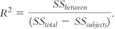
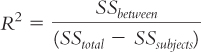
We divide the between-groups sum of squares by the difference between the total sum of squares and the subjects sum of squares. We remove the subjects sum of squares so we can determine the variability explained only by between-groups differences.

The calculations for R2 for a one-way within-groups ANOVA and a one-way between-groups ANOVA are similar. As before, the numerator is a measure of the variability that takes into account just the differences among means, SSbetween. The denominator, however, takes into account the total variability, SStotal, but removes the variability caused by differences among participants, SSsubjects. This enables us to determine the variability explained only by between-groups differences. The formula is:

image

EXAMPLE 11.6

Let’s apply this to the ANOVA we just conducted. We can use the statistics in the source table shown on page 304 to calculate R2:

image

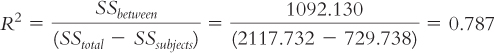
The conventions for R2 are the same as those shown in Table 11-12 (see page 294). This effect size of 0.79 is a very large effect: 79% of the variability in ratings of beer is explained by price.

Tukey HSD

EXAMPLE 11.7

We use the same procedure that we used for a one-way between-groups ANOVA, the Tukey HSD test: We calculate an HSD for each pair of means by first calculating the standard error:

image

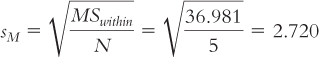
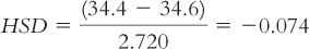
The standard error allows us to calculate HSD for each pair of means. Cheap beer (34.4) versus mid-range beer (34.6):

image

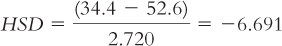
Cheap beer (34.4) versus high-end beer (52.6):

image

307

Mid-range beer (34.6) versus high-end beer (52.6):

image
image
Within-Groups Designs in Everyday Life We often use a within-groups design without even knowing it. A bride might use a within-groups design when she has all of her bridesmaids (the participants) try on several different possible dresses (the levels of the study). They would then choose the dress that is most flattering, on average, on the bridesmaids. We even have an innate understanding of order effects. A bride, for example, might ask her bridesmaids to try on the dress that she prefers either first or last (but not in the middle) so they’ll remember it better and be more likely to prefer it!
Megan Maloy/Getty Images

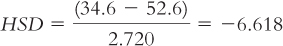
Now we look up the critical value in the q table in Appendix B. For a comparison of three means with within-groups degrees of freedom of 8 and a p level of 0.05, the cutoff q is 4.04. As before, the sign of each HSD does not matter.

The q table indicates two statistically significant differences for which the HSDs are beyond the critical values: −6.691 and −6.618. It appears that high-end beers elicit higher average ratings than cheap beers; high-end beers also elicit higher average ratings than mid-range beers. No statistically significant difference is found between cheap beers and mid-range beers.

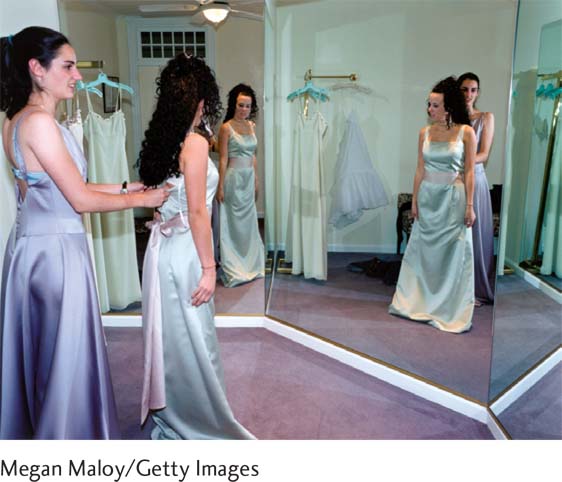
What might explain these differences? It’s not surprising that expensive beers came out ahead of cheap and midrange beers, but Fallows was surprised that no observable average difference was found between cheap and mid-range beers, which led to this advice that he gave to his beer-drinking colleagues: Buy high-end beer “when [you] want an individual glass of lager to be as good as it can be,” but buy cheap beer “at all other times, since it gives the maximum taste and social influence per dollar invested.” The mid-range beers? Not worth the money.

How much faith can we have in these findings? As behavioral scientists, we critically examine the design and procedures. Did the darker color of Sam Adams (the beer that received the highest average ratings) give it away as a high-end beer? The beers were labeled with letters (Budweiser was labeled with F). Yet, in line with many academic grading systems, the letter A has a positive connotation and F has a negative one. Were there order effects? Did the testers get more lenient (or critical) with every swallow? The panel of tasters was mostly Microsoft employees and was all men. Would we get different results for non-tech employees or with female participants? Science is a slow but sure way of knowing that depends on replication of experiments.

CHECK YOUR LEARNING

Reviewing the Concepts
  • It is recommended, as it is for other hypothesis tests, that we calculate a measure of effect size, R2, for a one-way within-groups ANOVA.

  • As with one-way between-groups ANOVA, if we are able to reject the null hypothesis with a one-way within-groups ANOVA, we’re not finished. We must conduct a post hoc test, such as a Tukey HSD test, to determine exactly which pairs of means are significantly different from one another.

Clarifying the Concepts 11-23 How does the calculation of the effect size R2 differ between the one-way within-groups ANOVA and the one-way between-groups ANOVA?
11-24 How does the calculation of the Tukey HSD differ between the one-way within-groups ANOVA and the one-way between-groups ANOVA?
Calculating the Statistics 11-25 A researcher measured the reaction time of six participants at three different times and found the mean reaction time at time 1 (M1 = 155.833), time 2 (M2 = 206.833), and time 3 (M3 = 251.667). The researcher rejected the null hypothesis after performing a one-way within-groups ANOVA. For the ANOVA, dfbetween = 2, dfwithin = 10, and MSwithin = 771.256.
  1. Calculate the HSD for each of the three mean comparisons.

  2. What is the critical value of q for this Tukey HSD test?

  3. For which comparisons do we reject the null hypothesis?

11-26 Use the following source table to calculate the effect size R2 for the one-way within-groups ANOVA.
Sources SS df MS F
Between 27,590.486 2 13,795.243 17.887
Subjects 16,812.189 5 3362.438 4.360
Within 7712.436 10 771.244
Total 52,115.111 17
Applying the Concepts 11-27 In Check Your Learning 11-21 and 11-22, we conducted an analysis of driver-experience ratings following test drives.
  1. Calculate R2 for this ANOVA, and state what size effect this is.

  2. Which follow-up tests are needed for this ANOVA, if any?

Solutions to these Check Your Learning questions can be found in Appendix D.