Exercises
Clarifying the Concepts
Question 14.1
| 14.1 |
What does regression add above and beyond what we learn from correlation? |
Question 14.2
| 14.2 |
How does the regression line relate to the correlation of the two variables? |
Question 14.3
| 14.3 |
Is there any difference between Ŷ and a predicted score for Y ? |
Question 14.4
| 14.4 |
What do each of the symbols stand for in the formula for the regression equation: zŶ = (rXY)(zX)? |
Question 14.5
| 14.5 |
The equation for a line is Ŷ = a + b(X). Define the symbols a and b. |
Question 14.6
| 14.6 |
What are the three steps to calculate the intercept? |
Question 14.7
| 14.7 |
When is the intercept not meaningful or useful? |
Question 14.8
| 14.8 |
What does the slope tell us? |
Question 14.9
| 14.9 |
Why do we also call the regression line the line of best fit? |
Question 14.10
| 14.10 |
How are the sign of the correlation coefficient and the sign of the slope related? |
Question 14.11
| 14.11 |
What is the difference between a small standard error of the estimate and a large one? |
Question 14.12
| 14.12 |
Why are explanations of the causes behind relations explored with regression limited in the same way they are with correlation? |
Question 14.13
| 14.13 |
What is the connection between regression to the mean and the bell- |
Question 14.14
| 14.14 |
Explain why the regression equation is a better source of predictions than is the mean. |
Question 14.15
| 14.15 |
What is the SStotal? |
Question 14.16
| 14.16 |
When drawing error lines between data points and the regression line, why is it important that these lines be perfectly vertical? |
Question 14.17
| 14.17 |
What are the basic steps to calculate the proportionate reduction in error? |
Question 14.18
| 14.18 |
What information does the proportionate reduction in error give us? |
Question 14.19
| 14.19 |
What is an orthogonal variable? |
Question 14.20
| 14.20 |
If you know the correlation coefficient, how can you determine the proportionate reduction in error? |
Question 14.21
| 14.21 |
Why is multiple regression often more useful than simple linear regression? |
Question 14.22
| 14.22 |
What is the difference between the symbol for the effect size for simple linear regression and the symbol for the effect size for multiple regression? |
Calculating the Statistics
Question 14.23
| 14.23 |
Using the following information, make a prediction for Y, given an X score of 2.9: Variable X: M = 1.9, SD = 0.6 Variable Y: M = 10, SD = 3.2 Pearson correlation of variables X and Y = 0.31
|
Question 14.24
| 14.24 |
Using the following information, make a prediction for Y, given an X score of 8: Variable X: M = 12, SD = 3 Variable Y: M = 74, SD = 18 Pearson correlation of variables X and Y = 0.46
|
Question 14.25
| 14.25 |
Let’s assume we know that age is related to bone density, with a Pearson correlation coefficient of –0.19. (Notice that the correlation is negative, indicating that bone density tends to be lower at older ages than at younger ages.) Assume we also know the following descriptive statistics: Age of people studied: 55 years on average, with a standard deviation of 12 years Bone density of people studied: 1000 mg/cm2 on average, with a standard deviation of 95 mg/cm2 Virginia is 76 years old. What would you predict her bone density to be? To answer this question, complete the following steps:
|
421
Question 14.26
| 14.26 |
Given the regression line Ŷ = –6 + 0.41(X), make predictions for each of the following:
|
Question 14.27
| 14.27 |
Given the regression line Ŷ = 49 – 0.18(X), make predictions for each of the following:
|
Question 14.28
| 14.28 |
Data are provided here with descriptive statistics, a correlation coefficient, and a regression equation: r = 0.426, Ŷ = 219.974 + 186.595(X).
Using this information, compute the following estimates of prediction error:
|
Question 14.29
| 14.29 |
Data are provided here with descriptive statistics, a correlation coefficient, and a regression equation: r = 0.52, Ŷ = 2.643 + 0.469(X).
Using this information, compute the following estimates of prediction error:
|
Question 14.30
| 14.30 |
Use this output from a multiple regression analysis to answer the following questions: 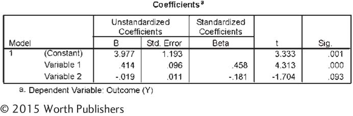
|
422
Question 14.31
| 14.31 |
Use this output from a multiple regression analysis to answer the following questions: 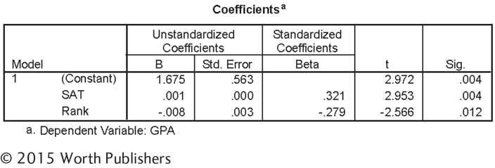
|
Applying the Concepts
Question 14.32
| 14.32 |
Weight, blood pressure, and regression: Several studies have found a correlation between weight and blood pressure.
|
Question 14.33
| 14.33 |
Temperature, hot chocolate sales, and prediction: Running a football stadium involves innumerable predictions. For example, when stocking up on food and beverages for sale at the game, it helps to have an idea of how much will be sold. In the football stadiums in colder climates, stadium managers use expected outdoor temperature to predict sales of hot chocolate.
|
Question 14.34
| 14.34 |
Age, hours studied, and prediction: In How It Works 13.2, we calculated the correlation coefficient between students’ age and number of hours they study per week. The correlation between these two variables is 0.49.
|
Question 14.35
| 14.35 |
Consideration of Future Consequences scale, z scores, and raw scores: A study of Consideration of Future Consequences (CFC) found a mean score of 3.51, with a standard deviation of 0.61, for the 664 students in the sample (Petrocelli, 2003).
|
Question 14.36
| 14.36 |
The GRE, z scores, and raw scores: The verbal subtest of the Graduate Record Examination (GRE) has a population mean of 500 and a population standard deviation of 100 by design (the quantitative subtest has the same mean and standard deviation).
|
Question 14.37
| 14.37 |
Hours studied, grade, and regression: A regression analysis of data from some of our statistics classes yielded the following regression equation for the independent variable (hours studied) and the dependent variable (grade point average [GPA]): Ŷ = 2.96 + 0.02(X).
|
423
Question 14.38
| 14.38 |
Precipitation, violence, and limitations of regression: Does the level of precipitation predict violence? Dubner and Levitt (2006b) reported on various studies that found links between rain and violence. They mentioned one study by Miguel, Satyanath, and Sergenti that found that decreased rain was linked with an increased likelihood of civil war across a number of African countries they examined. Referring to the study’s authors, Dubner and Levitt state, “The causal effect of a drought, they argue, was frighteningly strong.”
|
Question 14.39
| 14.39 |
Cola consumption, bone mineral density, and limitations of regression: Does one’s cola consumption predict one’s bone mineral density? Using regression analyses, nutrition researchers found that older women who drank more cola (but not more of other carbonated drinks) tended to have lower bone mineral density, a risk factor for osteoporosis (Tucker, Morita, Qiao, Hannan, Cupples, & Kiel, 2006). Cola intake, therefore, does seem to predict bone mineral density.
|
Question 14.40
| 14.40 |
Tutoring, mathematics performance, and problems with regression: A researcher conducted a study in which children with problems learning mathematics were offered the opportunity to purchase time with special tutors. The number of weeks that children met with their tutors varied from 1 to 20. He found that the number of weeks of tutoring predicted these children’s mathematics performance and recommended that parents of such children send them for tutoring.
|
Question 14.41
| 14.41 |
Anxiety, depression, and simple linear regression: We analyzed data from a larger data set that one of the authors used for previous research (Nolan, Flynn, & Garber, 2003). In the current analyses, we used regression to look at factors that predict anxiety over a 3- 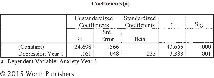
|
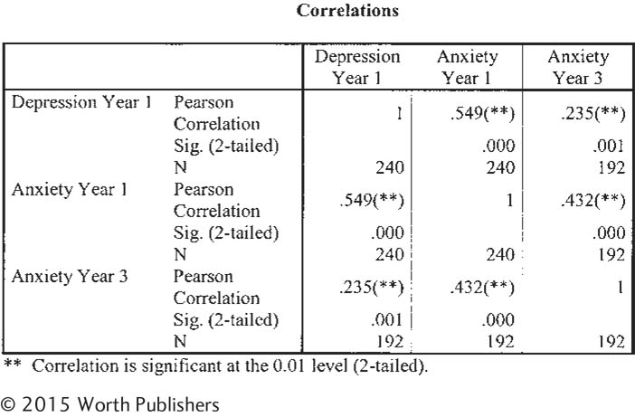
Question 14.42
| 14.42 |
Anxiety, depression, and multiple regression: We conducted a second regression analysis on the data from the previous exercise. In addition to depression at year 1, we included a second independent variable to predict anxiety at year 3. We also included anxiety at year 1. (We might expect that the best predictor of anxiety at a later point in time is one’s anxiety at an earlier point in time.) Here is the output for that analysis. 424 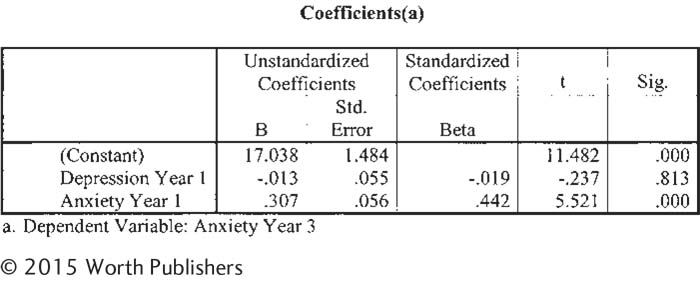
|
425
Question 14.43
| 14.43 |
Cohabitation, divorce, and prediction: A study by the Institute for Fiscal Studies (Goodman & Greaves, 2010) found that parents’ marital status when a child was born predicted the likelihood of the relationship’s demise. Parents who were cohabitating when their child was born had a 27% chance of breaking up by the time the child was 5, whereas those who were married when their child was born had a 9% chance of breaking up by the time the child was 5—
|
Question 14.44
| 14.44 |
Google, the flu, and third variables: The New York Times reported: “Several years ago, Google, aware of how many of us were sneezing and coughing, created a fancy equation on its Web site to figure out just how many people had influenza. The math works like this: people’s location + flu-
|
Question 14.45
| 14.45 |
Sugar, diabetes, and multiple regression: New York Times reporter Mark Bittman wrote: “A study published in the journal PLOS ONE links increased consumption of sugar with increased rates of diabetes by examining the data on sugar availability and the rate of diabetes in 175 countries over the past decade. And after accounting for many other factors, the researchers found that increased sugar in a population’s food supply was linked to higher diabetes rates independent of rates of obesity” (2013; http:/
|
Question 14.46
| 14.46 |
The age of a country, the level of concern for the environment, and multiple regression: Researchers analyzed the impact of the age of a country on the overall level of concern for the environment (Hershfield, Bang, & Weber, 2014). They noted that some countries—
|
426
Putting It All Together
Question 14.47
| 14.47 |
Age, hours studied, and regression: In How It Works 13.2, we calculated the correlation coefficient between students’ age and number of hours they study per week. The mean for age is 21, and the standard deviation is 1.789. The mean for hours studied is 14.2, and the standard deviation is 5.582. The correlation between these two variables is 0.49. Use the z score formula.
|
Question 14.48
| 14.48 |
Corporate political contributions, profits, and regression: Researchers studied whether corporate political contributions predicted profits (Cooper, Gulen, & Ovtchinnikov, 2007). From archival data, they determined how many political candidates each company supported with financial contributions, as well as each company’s profit in terms of a percentage. The accompanying table shows data for five companies. (Note: The data points are hypothetical but are based on averages for companies falling in the 2nd, 4th, 6th, and 8th deciles in terms of candidates supported. A decile is a range of 10%, so the 2nd decile includes those with percentiles between 10 and 19.9.)
|
427