15.1 CONDUCTING A CHI-SQUARE TEST FOR GOODNESS OF FIT

Gary Steinman (2006), an obstetrician and gynecologist, studied whether a woman’s diet could affect the likelihood that she would have twins. Insulin-like growth factor (IGF), often found in diets that include animal products like milk and beef, is hypothesized to lead to higher rates of twin births. Steinman wondered whether women who were vegans (those who eat neither meat nor dairy products) would have lower rates of twin births than would women who were vegetarians and consumed dairy products or women who ate meat. Steinman reported that, in the general population, 1.9% of births result in twins (without the aid of reproductive technologies). In Steinman’s study of 1042 vegans who gave birth (without reproductive technologies), four sets of twins were born. How can we use Steinman’s data to conduct the six steps of hypothesis testing for a chi-square test for goodness of fit?

Step 1: Population 1: Vegans who recently gave birth, like those whom we observed. Population 2: Vegans who recently gave birth who are like the general population of mostly nonvegans.

The comparison distribution is a chi-square distribution. The hypothesis test will be a chi-square test for goodness of fit because we have one nominal variable only. This study meets three of the four assumptions: (1) The one variable is nominal. (2) Every participant is in only one cell (a vegan woman is counted either as having twins or as having one child, or singleton). (3) There are far more than five times as many participants as cells (there are 1042 participants and only two cells). (4) The participants were not, however, randomly selected. We learn from the published research paper that participants were recruited with the assistance of “various vegan societies.” This limits our ability to generalize beyond vegan women like those in the sample.

Step 2: Null hypothesis: Vegan women give birth to twins at the same rate as the general population. Research hypothesis: Vegan women give birth to twins at a different rate than the general population.

Step 3: The comparison distribution is a chi-square distribution that has 1 degree of freedom: df_χ² = 2 – 1.

461

Step 4: The critical chi-square value, based on a p level of 0.05 and 1 degree of freedom, is 3.841, as seen in the curve in Figure 15-3.

Step 5: Observed (among vegan mothers)

Expected (based on the 1.9% rate in the general population)

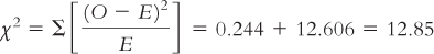
Step 6: Reject the null hypothesis; it appears that vegan mothers are less likely to have twins than are mothers in the general population.

The statistics, as reported in a journal article, would read:

χ² (1, N = 1042) = 12.85, p < 0.05

15.2 CONDUCTING A CHI-SQUARE TEST FOR INDEPENDENCE

Do people who move far from their hometown have a more exciting life? Since 1972, the General Social Survey (GSS) has asked approximately 40,000 adults in the United States numerous questions about their lives. During several years of the GSS, participants were asked, “In general, do you find life exciting, pretty routine, or dull?” (a variable called LIFE) and “When you were 16 years old, were you living in the same (city/town/country)?” (a variable called MOBILE16). How can we use these data to conduct the six steps of hypothesis testing for a chi-square test for independence?

In this case, there are two nominal variables. The independent variable is where a person lives relative to when he or she was 16 years old (same city, or same state but different city, or different state). The dependent variable is how the person finds life (exciting, routine, dull). Here are the data:

Step 1: Population 1: People like those in this sample. Population 2: People from a population in which a person’s characterization of life as exciting, routine, or dull does not depend on where that person is living relative to when he or she was 16 years old.

The comparison distribution is a chi-square distribution. The hypothesis test will be a chi-square test for independence because we have two nominal variables. This study meets all four assumptions: (1) The two variables are nominal. (2) Every participant is in only one cell. (3) There are more than five times as many participants as there are cells (there are 27,907 participants and 9 cells). (4) The GSS sample uses a form of random selection.

462

Step 2: Null hypothesis: The proportion of people who find life to be exciting, routine, or dull does not depend on where they live relative to where they lived when they were 16 years old. Research hypothesis: The proportion of people who find life exciting, routine, or dull differs depending on where they live relative to where they lived when they were 16 years old.

Step 3: The comparison distribution is a chi-square distribution with 4 degrees of freedom:

df_χ² = (k_row − 1)(k_column − 1) = (3 − 1)(3 − 1) = (2)(2) = 4

Step 4: The critical chi-square statistic, based on a p level of 0.05 and 4 degrees of freedom, is 9.488.

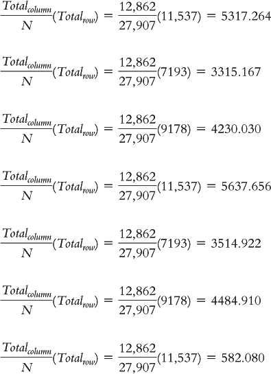
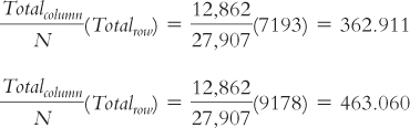
Step 5:

463

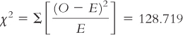
Step 6: Reject the null hypothesis. The calculated chi-square statistic exceeds the critical value. How exciting a person finds life does appear to vary with where the person lives relative to where he or she lived when he or she was 16 years old.

We would present these statistics in a journal article as: χ²(4, N = 27,907) = 128.72, p < 0.05.

15.3 CALCULATING CRAMÉR’S V

What is the effect size, Cramér’s V, for the chi-square test for independence we conducted in How It Works 15.2?

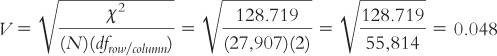
According to Cohen’s conventions, this is a small effect size. With this piece of information, we’d present the statistics in a journal article as:

χ²(4, N = 27,907) = 128.72 < 0.05, Cramér’s V = 0.05

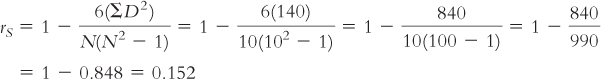
15.4 CALCULATING THE SPEARMAN RANK-ORDER CORRELATION COEFFICIENT

The accompanying table includes ranks for accomplishment-related national pride, along with numbers of medals won at the 2000 Sydney Olympics for 10 countries. (Of course, this might not be the best way to operationalize the variable of Olympic performance; perhaps we should be ranking Olympic medals per capita.) How can we calculate the Spearman correlation coefficient for these two variables—seen in the first two columns of the accompanying table—pride rank and Olympic medals?

First, we have to convert the numbers of Olympic medals to ranks. Then we can calculate the correlation coefficient.

464

ΣD2 = (0 + 25 + 25 + 1 + 25 + 9 + 9 + 36 + 9 + 1) = 140

15.5 CONDUCTING THE MANN–WHITNEY U TEST

The Mann–Whitney U test is the nonparametric version of the independent-samples t test, so it is useful when comparing the rankings of two different groups. For example, we can use rankings to ask: In which of two regions in the United States do political science graduate programs tend to have the best rankings—on the East Coast (E) or in the Midwest (M)? Here are data from U.S. News & World Report’s 2013 online rankings of graduate schools. These are the top 18 doctoral programs in political science that are either on the East Coast or in the Midwest. (There are 7 schools in other regions that are also in the top 25; they are omitted for the purposes of this example.) Schools listed at the same rank are tied.

465

How can we conduct a Mann–Whitney U test for this example? The independent variable is region of the country, and its levels are East Coast and Midwest. The dependent variable is U.S. News & World Report ranking.

Step 1: This study meets the first and third of the three assumptions: (1) There are ordinal data after we convert the data from scale to ordinal. (2) The researchers did not use random selection, so the ability to generalize beyond this sample is limited. (3) There are some ties, but we will assume that there are not so many as to render the results of the test invalid.

Step 2: Null hypothesis: Political science programs on the East Coast and those in the Midwest do not differ in national ranking. Research hypothesis: Political science programs on the East Coast and those in the Midwest differ in national ranking.

Step 3: There are 10 top political science programs on the East Coast and 8 in the Midwest.

Step 4: The cutoff, or critical value, for a Mann–Whitney U test with one group of 10 programs and one group of 8 programs, a p level of 0.05, and a two-tailed test is 17.

Step 5:

Before we continue, we sum the ranks for each group and add subscripts to indicate which group is which:

ΣR_E = (1 + 2 + 3.5 + 5 + 6 + 7 + 9.5 + 12.5 + 12.5 + 15.5) = 74.5

ΣR_M = (3.5 + 8 + 9.5 + 12.5 + 12.5 + 15.5 + 17 + 18) = 96.5

The formula for the first group is:

466

The formula for the second group is:

Step 6: For a Mann–Whitney U test, we compare only the smaller test statistic, 19.5, with the critical value, 17. This test statistic is not smaller than the critical value, so we fail to reject the null hypothesis. We cannot conclude that the two groups are different with respect to national rankings.

In a journal article, the statistics would read:

U = 19.5, p > 0.05