7.3 An Example of the z Test
The story of the doctor tasting tea inspired statisticians to use hypothesis testing as a way to understand the many mysteries of human behavior. In this section, we apply what we’ve learned about hypothesis testing—
EXAMPLE 7.5
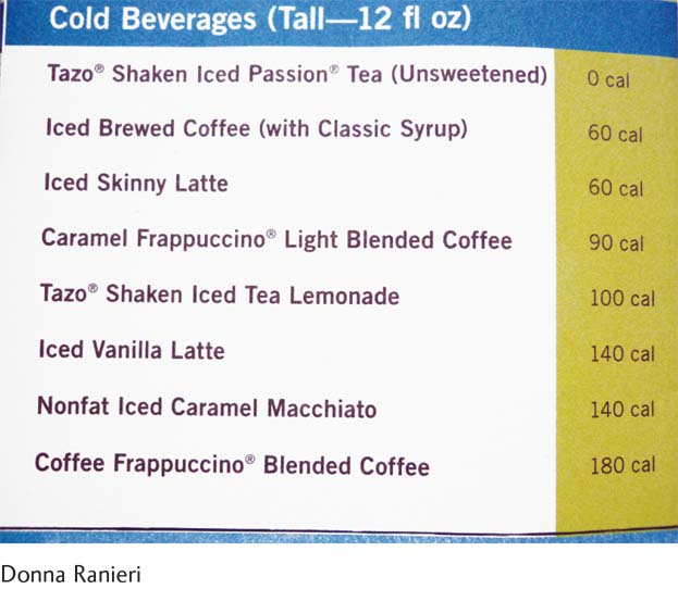
New York City was the first U.S. city to require that chain restaurants post calorie counts for all menu items. Shortly after the new law was implemented, the research team of Bollinger, Leslie, & Sorensen (2010) decided to test the law’s effectiveness. For more than a year, they gathered data on every transaction at Starbucks coffee shops in several cities. They determined a population mean of 247 calories in products purchased by customers at stores without calorie postings. Based on the range of 0 to 1208 calories in customer transactions, we estimate a standard deviation of approximately 201 calories, which we’ll use as the population standard deviation for this example.
The researchers also recorded calories for a sample in New York City after calories were posted on Starbucks menus. They reported a mean of 232 calories per purchase, a decrease of 6%. For the purposes of this example, we’ll assume a sample size of 1000. Here’s how to apply hypothesis testing when comparing a sample of customers at Starbucks with calories posted on their menus to the general population of customers at Starbucks without calories posted on their menus.
We’ll use the six steps of hypothesis testing to analyze the calorie data. These six steps will tell us if customers visiting a Starbucks with calories listed on the menu consume fewer calories, on average, than customers visiting a Starbucks without calories listed on the menu. In fact, we use the six-
171
STEP 1: Identify the populations, distribution, and assumptions.
First, we identify the populations, comparison distribution, and assumptions, which help us to determine the appropriate hypothesis test. The populations are (1) all customers at those Starbucks with calories posted on the menu (whether or not the customers are in the sample) and (2) all customers at those Starbucks without calories posted on the menu. Because we are studying a sample rather than an individual, the comparison distribution is a distribution of means. We compare the mean of the sample of 1000 people visiting those Starbucks that have calories posted on the menu (selected from the population of all people visiting those Starbucks with calories posted) to a distribution of all possible means of samples of 1000 people (selected from the population of all people visiting those Starbucks that don’t have calories posted on the menu). The hypothesis test will be a z test because we have only one sample and we know the mean and the standard deviation of the population from the published norms.
Now let’s examine the assumptions for a z test. (1) The data are on a scale measure, calories. (2) We do not know whether sample participants were selected randomly from among all people visiting those Starbucks with calories posted on the menu. If they were not, the ability to generalize beyond this sample to other Starbucks customers would be limited. (3) The comparison distribution should be normal. The individual data points are likely to be positively skewed because the minimum score of 0 is much closer to the mean of 247 than it is to the maximum score of 1208. However, we have a sample size of 1000, which is greater than 30; so based on the central limit theorem, we know that the comparison distribution—
Summary: Population 1: All customers at those Starbucks that have calories posted on the menu. Population 2: All customers at those Starbucks that don’t have calories posted on the menu.
The comparison distribution will be a distribution of means. The hypothesis test will be a z test because we have only one sample and we know the population mean and standard deviation. This study meets two of the three assumptions and may meet the third. The dependent variable is scale. In addition, there are more than 30 participants in the sample, indicating that the comparison distribution will be normal. We do not know whether the sample was randomly selected, however, so we must be cautious when generalizing.
STEP 2: State the null and research hypotheses.
Next we state the null and research hypotheses in words and in symbols. Remember, hypotheses are always about populations, not samples. In most forms of hypothesis testing, there are two possible sets of hypotheses: directional (predicting either an increase or a decrease, but not both) or nondirectional (predicting a difference in either direction).
The first possible set of hypotheses is directional. The null hypothesis is that customers at those Starbucks that have calories posted on the menu do not consume fewer mean calories than customers at those Starbucks that don’t have calories posted on the menu; in other words, they could consume the same or more mean calories, but not fewer. The research hypothesis is that customers at those Starbucks that have calories posted on the menu consume fewer mean calories than do customers at Starbucks that don’t have calories posted on the menu. (Note that the direction of the hypotheses could be reversed.)
The symbol for the null hypothesis is H0. The symbol for the research hypothesis is H1. Throughout this text, we use μ for the mean because hypotheses are about populations and their parameters, not about samples and their statistics. So, in symbolic notation, the hypotheses are:
172
H0: μ1 ≥ μ2
H1: μ1 < μ2
For the null hypothesis, the symbolic notation says that the mean calories consumed by those in population 1, customers at those Starbucks with calories posted on the menu, is not lower than the mean calories consumed by those in population 2, customers at those Starbucks without calories posted on the menu. For the research hypothesis, the symbolic notation says that the mean calories consumed by those in population 1 is lower than the mean calories consumed by those in population 2.
A one-
tailed test is a hypothesis test in which the research hypothesis is directional, positing either a mean decrease or a mean increase in the dependent variable, but not both, as a result of the independent variable.
This hypothesis test is considered a one-
The second set of hypotheses is nondirectional. The null hypothesis states that customers at Starbucks with posted calories (whether in the sample or not) consume the same number of calories, on average, as customers at Starbucks without posted calories. The research hypothesis is that customers at Starbucks with posted calories (whether in the sample or not) consume a different average number of calories than do customers at Starbucks without posted calories. The means of the two populations are posited to be different, but neither mean is predicted to be lower or higher.
The hypotheses in symbols would be:
H0: μ1 = μ2
H1: μ1 ≠ μ2
For the null hypothesis, the symbolic notation says that the mean number of calories consumed by those in population 1 is the same as the mean number of calories consumed by those in population 2. For the research hypothesis, the symbolic notation says that the mean number of calories consumed by those in population 1 is different from the mean number of calories consumed by those in population 2.
A two-
tailed test is a hypothesis test in which the research hypothesis does not indicate a direction of the mean difference or change in the dependent variable, but merely indicates that there will be a mean difference.
This hypothesis test is considered a two-
MASTERING THE CONCEPT
7-
Summary: Null hypothesis: Customers at those Starbucks that have calories posted on the menu consume the same number of calories, on average, as do customers at Starbucks that don’t have calories posted on the menu—
173
STEP 3: Determine the characteristics of the comparison distribution.
Now we determine the characteristics that describe the distribution with which we will compare the sample. For z tests, we must know the mean and the standard error of the population of scores; the standard error for samples of this size is calculated from the standard deviation of the population of scores. Here, the population mean for the number of calories consumed by the general population of Starbucks customers is 247, and the standard deviation is 201. The sample size is 1000. Because we use a sample mean in hypothesis testing, rather than a single score, we must use the standard error of the mean instead of the population standard deviation (of the scores). The characteristics of the comparison distribution are determined as follows:
μM = μ = 247
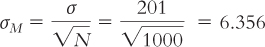
Summary: μM = 247; σM = 6.356
STEP 4: Determine the critical values, or cutoffs.
Next we determine the critical values, or cutoffs, to which we can compare the test statistic. As stated previously, the research convention is to set the cutoffs to a p level of 0.05. For a two-
We know that 50% of the curve falls above the mean, and we know that 2.5% falls above the relevant z statistic. By subtracting (50% – 2.5% = 47.5%), we determine that 47.5% of the curve falls between the mean and the relevant z statistic. When we look up this percentage on the z table, we find a z statistic of 1.96. So the critical values are –1.96 and 1.96 (Figure 7-10).
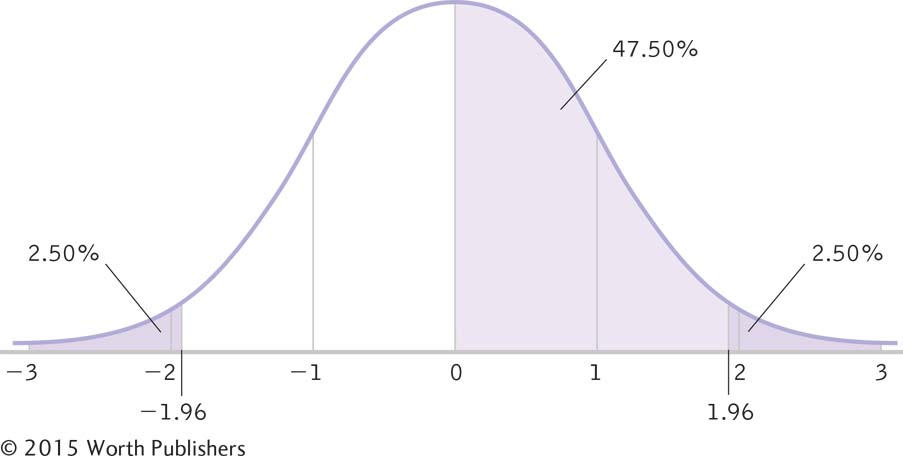
Determining Critical Values for a z Distribution
We typically determine critical values in terms of z statistics so we can easily compare a test statistic to determine whether it is beyond the critical values. Here z scores of –1.96 and 1.96 indicate the most extreme 5% of the distribution, 2.5% in each tail.
174
Summary: The cutoff z statistics are –1.96 and 1.96.
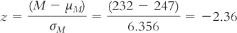
STEP 5: Calculate the test statistic.
In step 5, we calculate the test statistic, in this case a z statistic, to find out what the data really say. We use the mean and standard error calculated in step 3:
Summary: 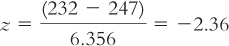
STEP 6: Make a decision.
Finally, we compare the test statistic to the critical values. We add the test statistic to the drawing of the curve that includes the critical z statistics (Figure 7-11). If the test statistic is in the critical region, we can reject the null hypothesis. In this example, the test statistic, –2.36, is in the critical region, so we reject the null hypothesis. An examination of the means tells us that the mean number of calories consumed by customers at those Starbucks with calories posted on the menu is lower than the mean number of calories consumed by customers at those Starbucks with no calories posted. So, even though we had nondirectional hypotheses, we can report the direction of the finding—
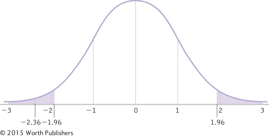
Making a Decision
To decide whether to reject the null hypothesis, we compare the test statistic to the critical values. In this instance, the z score of –2.36 is beyond the critical value of –1.96, so we reject the null hypothesis. Customers at those Starbucks with calories posted on the menu consume fewer calories, on average, than do customers at those Starbucks without posted calories.
If the test statistic is not beyond the cutoffs, we fail to reject the null hypothesis. This means that we can only conclude that there is no evidence from this study to support the research hypothesis. There might be a real mean difference that is not extreme enough to be picked up by the hypothesis test. We just can’t know.
Summary: We reject the null hypothesis. It appears that fewer calories are consumed, on average, by customers at Starbucks that post calories on the menus than by customers at Starbucks that do not post calories on the menu.
The researchers who conducted this study concluded that the posting of calories by restaurants does indeed seem to be beneficial. The 6% reduction may seem small, they admit, but they report that the reduction was larger—
175
CHECK YOUR LEARNING
| Reviewing the Concepts |
|
|
| Clarifying the Concepts | 7- |
What does it mean to say a test is directional or nondirectional? |
| Calculating the Statistics | 7- |
Calculate the characteristics ( μM and σM) of a comparison distribution for a sample mean based on 53 participants when the population has a mean of 1090 and a standard deviation of 87. |
| 7- |
Calculate the z statistic for a sample mean of 1094 based on the sample of 53 people when μ = 1090 and σ = 87. | |
| Applying the Concepts | 7- |
According to the Web site for the Coffee Research Institute (http:/ |
Solutions to these Check Your Learning questions can be found in Appendix D.