nolanheinzen3e

Chapter 9

9.1 We should use a t distribution when we do not know the population standard deviation and are comparing two groups.
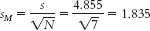
9.3 For both tests, standard error is calculated as the standard deviation divided by the square root of N. For the z test, the population standard deviation is calculated with N in the denominator. For the t test, the standard deviation for the population is estimated by dividing the sum of squared deviations by N − 1.
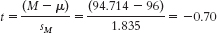
9.5t stands for the t statistic, M is the sample mean, μ_M is the mean of the distribution of means, and _sM is the standard error as estimated from a sample.
9.7Free to vary refers to the number of scores that can take on different values if a given parameter is known.
9.9 As the sample size increases, we can feel more confident in the estimate of the variability in the population. Remember, this estimate of variability (s) is calculated with N + 1 in the denominator in order to inflate the estimate somewhat. As the sample increases from 10 to 100, for example, and then up to 1000, subtracting 1 from N has less of an impact on the overall calculation. As this happens, the t distributions approach the z distribution, where we in fact knew the population standard deviation and did not need to estimate it.
9.11 A dot plot depicts the distribution of the sample data and thus provides information similar to that provided by a histogram. The dot plot, however, contains a separate dot for each observation.
9.13
- a. First we need to calculate the mean:
  
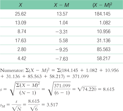
  We then calculate the deviation of each score from the mean and the square of that deviation.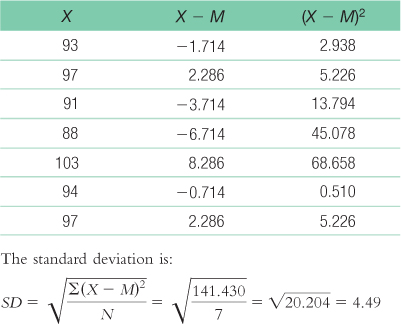
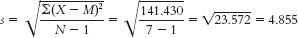
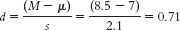
- b. When estimating the population variability, we calculate s:
- c.
- d.
9.15
- a. Because 73 df is not on the table, we go to 60 df (we do not go to the closest value, which would be 80, because we want to be conservative and go to the next-lowest value for df) to find the critical value of 1.296 in the upper tail. If we are looking in the lower tail, the critical value is −1.296.
- b. ±1.984
- c. Either −2.438 or 2.438
9.17
- a. This is a two-tailed test with df = 25, so the critical t values are ±2.060.
- b. df = 17, so the critical t value is +2.567, assuming you’re anticipating an increase in marital satisfaction.
- c. df = 33, so the critical t values are ±2.043.
9.19
- a.
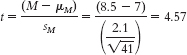
- b. M_lower = −t(s_M) + M_sample = −2.705(0.328) + 8.5 = 7.61
  M_upper = t(s_M) + M_sample = 2.705(0.328) + 8.5 = 9.39
- c.
9.21
- a. ±1.96
- b. Either −2.33 or +2.33, depending on the tail of interest
- c. ±1.96
- d. The critical z values are lower than the critical t values, making it easier to reject the null hypothesis when conducting a z test. Decisions using the t distributions are more conservative because of the chance that the population standard deviation may have been poorly estimated.
9.23
- a. Step 1: Population 1 is male U.S. Marines following a month-long training exercise. Population 2 is college men. The comparison distribution will be a distribution of means. The hypothesis test will be a single-sample t test because we have only one sample and we know the population mean but not the standard deviation. This study meets one of the three assumptions and may meet another. The dependent variable, anger, appears to be scale. The data were not likely randomly selected, so we must be cautious with respect to generalizing to all Marines who complete this training. We do not know whether the population is normally distributed, and there are not at least 30 participants. However, the data from the sample do not suggest a skewed distribution.
  Step 2: Null hypothesis: Male U.S. Marines after a month- long training exercise have the same average anger levels as college men—H₀: μ₁ + μ₂.
  Research hypothesis: Male U.S. Marines after a month-long training exercise have different average anger levels than college men—H₁: μ₁ ≠ μ₂.
  Step 3: μ_M = μ + 8.90; s_M + 0.494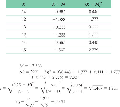
  
  C-27
  Step 4: df = N − 1 = 6 − 1 = 5; the critical values, based on 5 degrees of freedom, a p level of 0.05, and a two-tailed test, are −2.571 and 2.571. (Note: It is helpful to draw a curve that includes these cutoffs.)
  Step 5: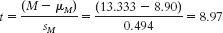
  (Note: It is helpful to add this t statistic to the curve that you drew in step 4.)
  Step 6: Reject the null hypothesis. It appears that male U.S. Marines just after a month-long training exercise have higher average anger levels than college men; t(5) = 8.97, p < 0.05.
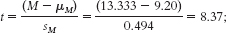
- b. reject the null hypothesis; it appears that male U.S. Marines just after a month-long training exercise have higher average anger levels than adult men; tX5C = 8.37, p < 0.05.
- c. 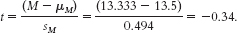Fail to reject the null hypothesis; we conclude that there is no evidence from this study to support the research hypothesis; t(5) = −0.34, p < 0.05.
- d. We can conclude that Marines’ anger scores just after high-altitude, cold-weather training are, on average, higher than those of college men and adult men. We cannot conclude, however, that they are different, on average, than those of male psychiatric outpatients. With respect to the latter difference, we can only conclude that there is no evidence to support that there is a difference between Marines’ mean anger scores and those of male psychiatric outpatients.
9.25
- a.
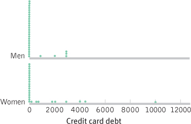
- b. The distributions are similar in that 0 is the modal amount of credit card debt for both women and men. The majority of participants in this study reported no credit card debt. Both distributions are positively skewed, particularly the distribution for women. Moreover, the distribution for women shows a potential outlier.
9.27
- a. The appropriate mean: μ_M = μ = 11.72 The calculations for the appropriate standard deviation (in this case, standard error, s_M) are:
- b.
- c. There are several possible answers to this question. Among the hypotheses that could be examined are whether the length of stay on death row depends on gender, race, or age. Specifically, given prior evidence of a racial bias in the implementation of the death penalty, we might hypothesize that black and Hispanic prisoners have shorter times to execution than do prisoners overall.
- d. We would need to know the population standard deviation. If we were really interested in this, we could calculate the standard deviation from the entire online execution list.
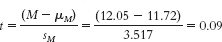
- e. The null hypothesis states that the average time spent on death row in recent years is equal to what it has been historically (no change)—H₀: μ₁ = μ₂. The research hypothesis is that there has been a change in the average time spent on death row—H₁: μ₁ ≠ μ₂.
- f. The t statistic we calculated was 0.09. The critical t values for a two-tailed test, alpha or p of 0.05 and df of 5, are ±2.571. We fail to reject the null hypothesis and conclude that we do not have sufficient evidence to indicate a change in time spent on death row.
- g.
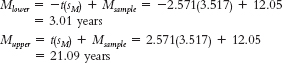
- h. Because the population mean of 11.72 years is within the very large range of the confidence interval, we fail to reject the null hypothesis. This confidence interval is so large that it is not useful. The large size of the confidence interval is due to the large variability in the sample (s_M) and the small sample size (resulting in a large critical t value).
- i.
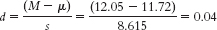
- j. This is a small effect.

C-28