Chapter 12
- 12.1 An ANOVA is a hypothesis test with at least one nominal independent variable (with at least three total groups) and a scale-
dependent variable. - 12.3 Between-
groups variance is an estimate of the population variance based on the differences among the means; within- groups variance is an estimate of the population variance based on the differences within each of the three (or more) sample distributions. - 12.5 The three assumptions are that the participants were randomly selected, the underlying populations are normally distributed, and the underlying variances of the different conditions are similar, or homoscedastic.
- 12.7 The F statistic is calculated as the ratio of two variances. Variability, and the variance measure of it, is always positive—
it always exists. Variance is calculated as the sum of squared deviations, and squaring both positive and negative values makes them positive. - 12.9 With sums of squares, we add up all the squared values. Deviations from the mean always sum to 0. By squaring these deviations, we can sum them and they will not sum to 0. Sums of squares are measures of variability of scores from the mean.
- 12.11 The grand mean is the mean of every score in a study, regardless of which sample the score came from.
- 12.13 Cohen’s d; R2
- 12.15Post hoc means “after this.” These tests are needed when an ANOVA is significant and we want to discover where the significant differences exist between the groups.
- 12.17
- a. Standard error is wrong. The professor is reporting the spread for a distribution of scores, the standard deviation.
- b. t statistic is wrong. We do not use the population standard deviation to calculate a t statistic. The sentence should say z statistic instead.
- c. Parameters is wrong. Parameters are numbers that describe populations, not samples. The researcher calculated the statistics.
- d. z statistic is wrong. Evelyn is comparing two means; thus, she would have calculated a t statistic.
- 12.19 When performing Bonferroni post hoc comparisons, you adjust the p level by dividing the p level for the experiment by the number of comparisons you want to make. You then calculate multiple t tests—
one for each two- group comparison you make— and compare the p value for each test to the new Bonferroni- adjusted p level. - 12.21
- a. dfbetween = Ngroups − 1 = 3 − 1 = 2
- b. dfwithin = df1 + df2 + … + dflast = (4 − 1) + (3 − 1) + (5 − 1) = 3 + 2 + 4 = 9
- c. dftotal = dfbetween + dfwithin = 2 + 9 = 11
- d. The critical value for a between-
groups degrees of freedom of 2 and a within- groups degrees of freedom of 9 at a p level of 0.05 is 4.26. C-
36 - e.
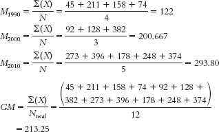
- f. (Note: The total sum of squares may not exactly equal the sum of the between-
groups and within- groups sums of squares because of rounding decisions.)
The total sum of squares is calculated here as SStotal = Σ(X − GM)2: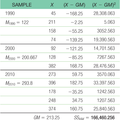
- g. The within-
groups sum of squares is calculated here as SSwithin = Σ(X − M)2: 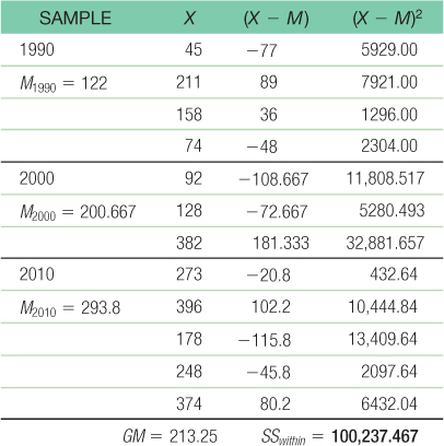
- h. The between-
groups sum of squares is calculated here as SSbetween = Σ(M − GM)2: 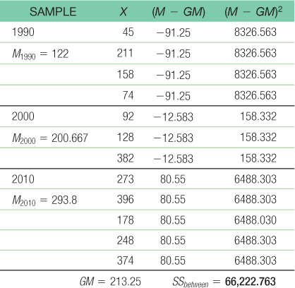
- i.
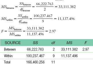
- j. Effect size is calculated as
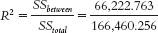 = 0.40. According to Cohen’s conventions for R2, this is a very large effect.
- 12.23
- a.
- b.

- c.

- a.
- 12.25
SOURCE SS df MS F Between 43 2 21.500 2.66 Within 89 11 8.091 Total 132 13 - 12.27 With four groups, there would be a total of six different comparisons.
- 12.29 With seven groups, there would be a total of 21 different comparisons. The first group would be compared with groups 2, 3, 4, 5, 6, and 7. The second group would be compared with groups 3, 4, 5, 6, and 7. The third group would be compared with groups 4, 5, 6, and 7. The fourth group would be compared with groups 5, 6, and 7. The fifth group would be compared with groups 6 and 7. And the sixth group would be compared with group 7.
C-
37 - 12.31
- a. The independent variable is type of program. The levels are The Daily Show and network news. The dependent variable is the amount of substantive video and audio reporting per second.
- b. The hypothesis test that Fox would use is an independent-
samples t test. - c. The independent variable is still type of program, but now the levels are The Daily Show, network news, and cable news. The hypothesis test would be a one-
way between- groups ANOVA.
- 12.33
- a. A t distribution; we are comparing the mean IQ of a sample of 10 to the population mean of 100; this student knows only the population mean—
not the population standard deviation. - b. An F distribution; we are comparing the mean ratings of four samples—
families with no books visible, with only children’s books visible, with only adult books visible, and with both types of books visible. - c. A t distribution; we are comparing the average vocabulary of two groups.
- a. A t distribution; we are comparing the mean IQ of a sample of 10 to the population mean of 100; this student knows only the population mean—
- 12.35
- a. The independent variable in this case is the type of program in which students were enrolled; the levels were arts and sciences, education, law, and business. Because every student is enrolled in only one program, the researcher would use a one-
way between- groups ANOVA. - b. Now the independent variable is year, with levels of first, second, or third. Because the same participants are repeatedly measured, the researcher would use a one-
way within- groups ANOVA. - c. The independent variable in this case is type of degree, and its levels are master’s, doctoral, and professional. Because every student is in only one type of degree program, the researcher would use a one-
way between- groups ANOVA. - d. The independent variable in this case is stage of training, and its levels are master’s, doctoral, and postdoctoral. Because the same students are repeatedly measured, the researcher would use a one-
way within- groups ANOVA.
- a. The independent variable in this case is the type of program in which students were enrolled; the levels were arts and sciences, education, law, and business. Because every student is enrolled in only one program, the researcher would use a one-
- 12.37
- a. The independent variable is political viewpoint, with the levels Republican, Democrat, and neither.
- b. The dependent variable is religiosity.
- c. The populations are all Republicans, all Democrats, and all who categorize themselves as neither. The samples are the Republicans, Democrats, and people who say they are neither among the 180 students.
- d. Because every student identified only one type of political viewpoint, the researcher would use a one-
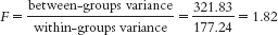
way between- groups ANOVA. No participant could be in more than one level of the independent variable. - e. First, we would calculate the between-
groups variance. This involves calculating a measure of variability among the three sample means— the religiosity scores of the Republicans, Democrats, and others. Then we would calculate the within- groups variance; this is essentially an average of the variability within each of the three samples. Finally, we would divide the between- groups variance by the within- groups variance. If the variability among the means is much larger than the variability within each sample, this provides evidence that the means are different from one another.
- 12.39
- a.
- b.

- c. The “Sig.” for t is the same as that for the ANOVA, 0.005, because the F distribution reduces to the t distribution when we are dealing with two groups.
- a.
- 12.41
- a. The independent variable is instructor self-
disclosure, which is a nominal variable with three levels— high, medium, and low self- disclosure. - b. The first dependent variable mentioned is levels of motivation, which is a scale variable.
- c. This is a between-
groups design because students are only exposed to one of the three types of instructor self- disclosure via the Facebook pages. - d. A one-
way between- subjects ANOVA would be used to analyze the data. - e. This is a true experiment as participants were randomly assigned to levels of a manipulated independent variable. This means that the researchers can draw a causal conclusion. That is, they can conclude that high self-
disclosure causes “higher levels of motivation and affective learning and a more positive classroom climate,” as compared with low and medium levels of self- disclosure.
- a. The independent variable is instructor self-
- 12.43
- a. The independent variable is languages spoken, which is a nominal variable with four levels—
monolingual (English), bilingual (Spanish- English), bilingual (French- English), and bilingual (Chinese- English). The dependent variable is vocabulary skills as assessed by the PPVT, a scale variable. - b. We know that the finding is statistically significant because the p value of 0.0001 is less than the typical cutoff p level of 0.05.
- c. The findings from the one-
way ANOVA only tell us that there is at least one difference among the groups but not which specific groups are statistically significantly different from each other. - d. The Bonferroni test is a more conservative post hoc test. It is used to determine a critical value that is stricter than that based on a p level of .05. We can use this more conservative critical value to determine whether we can reject the null hypothesis when comparing the four levels of the independent variable.
- e. Statistically significant mean differences between mean vocabulary scores exist between the monolingual children and the bilingual (Chinese-
English) children and between the monolingual children and the bilingual (French- English) children. They also exist between the bilingual (Spanish- English) children and the bilingual (Chinese- English) children and between the bilingual (Spanish- English) children and the bilingual (French- English) children. However, the monolingual children and bilingual (Spanish- English) children did not statistically significantly differ from each other, on average, nor did the bilingual (Chinese- English) and bilingual (French- English) children statistically significantly differ from each other, on average.
- a. The independent variable is languages spoken, which is a nominal variable with four levels—
- 12.45
- a. Level of trust in the leader is the independent variable. It has three levels: low, moderate, and high.
C-
38 - b. The dependent variable is level of agreement with a policy supported by the leader or supervisor.
- c. Step 1: Population 1 is employees with low trust in their leader. Population 2 is employees with moderate trust in their leader. Population 3 is employees with high trust in their leader. The comparison distribution will be an F distribution. The hypothesis test will be a one-
way between- groups ANOVA. We do not know if employees were randomly selected. We also do not know if the underlying distributions are normal, and the sample sizes are small so we must proceed with caution. To check the final assumption, that we have homoscedastic variances, we will calculate variance for each group. Because the largest variance, 111, is much more than twice as large as the smallest variance, we can conclude we have heteroscedastic variances. Violation of this third assumption of homoscedastic samples means we should proceed with caution. Because these data are intended to give you practice calculating statistics, proceed with your analyses. When conducting real research, we would want to have much larger sample sizes and to more carefully consider meeting the assumptions.SAMPLE LOW TRUST MODERATE TRUST HIGH TRUST Squared deviations 16 100 3.063 1 121 18.063 4 1 60.063 25 27.563 Sum of squares 46 222 108.752 N − 1 3 2 3 Variance 15.33 111 36.25
Step 2: Null hypothesis: There are no mean differences between these three groups: The mean level of agreement with a policy does not vary across the three trust levels—H0: μ1 = μ2 = μ3.
Research hypothesis: There are mean differences between some or all of these groups: the mean level of agreement depends on trust.
Step 3: dfbetween = Ngroups − 1 = 3 − 1 = 2
dfwithin = df1 + df2 + … + dflast = (4 − 1) + (3 − 1) + (4 − 1) = 3 + 2 + 3 = 8
dftotal = dfbetween + dfwithin = 2 + 8 = 10
The comparison distribution will be an F distribution with 2 and 8 degrees of freedom.
Step 4: The critical value for the F statistic based on a p level of 0.05 is 4.46.
Step 5: GM = 21.727
Total sum of squares is calculated here as SStotal = Σ(X − GM)2:Within-
groups sum of squares is calculated here as SSwithin = Σ(X − M)2: Between-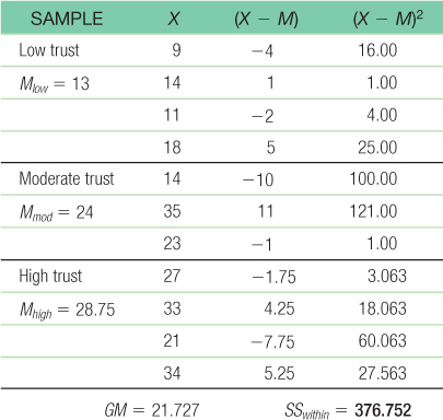
groups sum of squares is calculated here as SSbetween = Σ(M − GM)2: 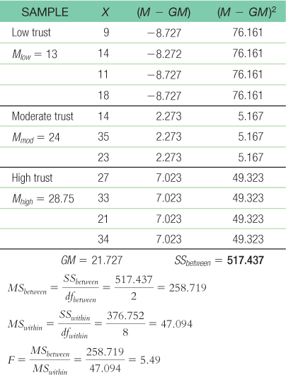
C-
39 Step 6: The F statistic, 5.49, is beyond the cutoff of 4.46, so we can reject the null hypothesis. The mean level of agreement with a policy supported by a supervisor varies across level of trust in that supervisor. Remember, the research design and data did not meet the three assumptions of this statistical test, so we should be careful in interpreting this finding.SOURCE SS df MS F Between 517.437 2 258.719 5.49 Within 376.752 8 47.094 Total 894.187 10 - d. F(2,8) = 5.49, p < 0.05; Note: We would include the actual p value if we used software to conduct this analysis.
- e. Because there are unequal sample sizes, we must calculate a weighted sample size.
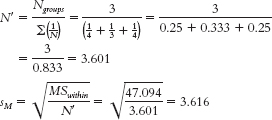
Now we can compare the three groups.
Low trust (M = 13) versus moderate trust (M = 24):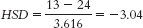
Low trust (M = 13) versus high trust (M = 28.75):
Moderate trust (M = 24) versus high trust (M = 28.75):
According to the q table, the critical value is 4.04 for a p level of 0.05 when we are comparing three groups and have within-groups degrees of freedom of 8. We obtained one q value (−4.36) that exceeds this cutoff. Based on the calculations, there is a statistically significant difference between the mean level of agreement by employees with low trust in their supervisors compared to those with high trust. Because the sample sizes here were so small and we did not meet the three assumptions of ANOVA, we should be careful in making strong statements about this finding. In fact, these preliminary findings would encourage additional research. - f. It is not possible to conduct a t test in this situation because there are more than two groups or levels of the independent variable.
- g. It is not possible to conduct this study with a within-
groups design because participants cannot be in more than one of the groups or levels of the independent variable. In other words, an employee has only one level of trust in his or her supervisor.
- a. Level of trust in the leader is the independent variable. It has three levels: low, moderate, and high.