Chapter 13
- 13.1 The four assumptions are that (1) the data are randomly selected; (2) the underlying population distributions are normal; (3) the variability is similar across groups, or homoscedasticity; and (4) there are no order effects.
- 13.3 The “subjects” variability is noise in the data caused by each participant’s personal variability compared with the other participants. It is calculated by comparing each person’s mean response across all levels of the independent variable with the grand mean, the overall mean response across all levels of the independent variable.
- 13.5 Counterbalancing involves exposing participants to the different levels of the independent variable in different orders.
- 13.7 To calculate the sum of squares for subjects, we first calculate an average of each participant’s scores across the levels of the independent variable. Then we subtract the grand mean from each participant’s mean. We repeat this subtraction for each score the participant has—
that is, for as many times as there are levels of the independent variable. Once we have the deviation scores, we square each of them and then sum the squared deviations to get the sum of squares for participants. - 13.9 If we have a between-
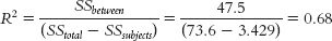
groups study in which different people are participating in the different conditions, then we can turn it into a within- groups study by having all the people in the sample participate in all the conditions. - 13.11 The calculations for R2 for a one-
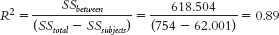
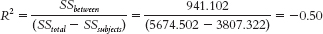
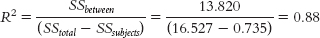
way within- groups ANOVA and a one- way between- groups ANOVA are similar. In both one- way ANOVAs, the numerator is a measure of the variability that takes into account just the differences among means, SSbetween. The denominator, however, is different for the within- groups ANOVA, as it takes into account the total variability, SStotal, similarly to the between- groups ANOVA, but removes the variability due to differences among participants, SSsubjects. This enables us to determine the variability explained only by between- groups differences. - 13.13
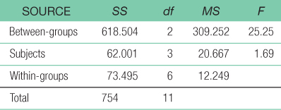
- a. dfbetween = Ngroups − 1 = 3 − 1 = 2
- b. dfsubjects = n − 1 = 4 − 1 = 3
- c. dfwithin = (dfbetween)(dfsubjects) = (2)(3) = 6
- d. dftotal = dfbetween + dfsubjects + dfwithin = 2 + 3 + 6 = 11, or we can calculate it as dftotal = Ntotal − 1 = 12 − 1 = 11
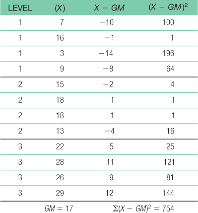
- e. SStotal = Σ(X − GM)2 = 754
C-
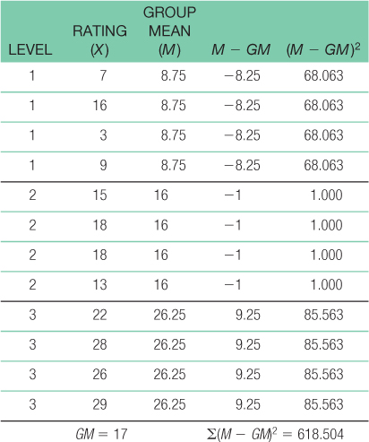
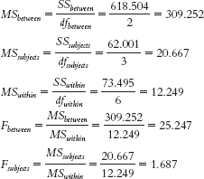
40 - f. SSbetween = Σ(M − GM)2 = 618.504
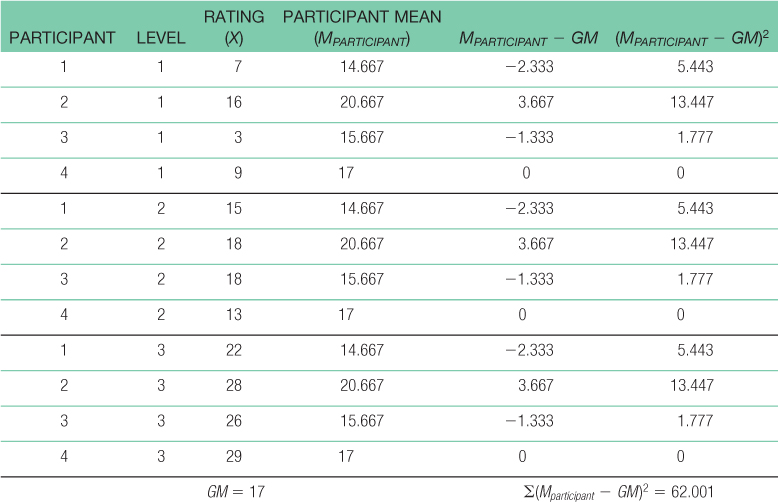
- g. SSsubjects = Σ(Mparticipant − GM)2 = 62.001
- h. SSwithin = SStotal − SSbetween − SSsubjects = 754 − 618.504 − 62.001 = 73.495
- i.
- j.
- k.
The Tukey HSD statistic comparing level 1 and level 3 would be: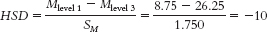
C-
41 - 13.15
- a.
SOURCE SS df MS F Between 941.102 2 470.551 10.16 Subjects 3807.322 10 380.732 8.22 Within 926.078 20 46.304 Total 5674.502 32 - b.
- a.
- 13.17
- a. Null hypothesis: People experience the same mean amount of fear across all three levels of dog size—
H0: μ1 = μ2 = μ3.Research hypothesis: People do not experience the same mean amount of fear across all three levels of dog size. - b. We do not know how the participants were selected, so the first assumption of random selection might not be met. We do not know how the dogs were presented to the participants, so we cannot assess whether order effects are present.
- c. The effect size was 0.89, which is a large effect. This indicates that the effect might be important, meaning the size of a dog might have a large impact on the amount of fear people experience.
- d. The Tukey HSD test statistic was −10. According to the q statistic table, the critical value for the Tukey HSD when there are 6 within-
groups degrees of freedom and three treatment levels is 4.34. We can conclude that the mean difference in fear when a small versus large dog is presented is statistically significant, with the large dog evoking greater fear.
- a. Null hypothesis: People experience the same mean amount of fear across all three levels of dog size—
- 13.19
- a. Step 5: We must first calculate df and SS to fill in the source table.
dfbetween = Ngroups − 1 = 2
dfsubjects = n − 1 = 4
dfwithin = (dfbetween)(dfsubjects) = 8
dftotal = Ntotal − 1 = 14
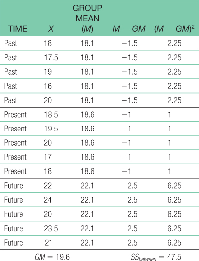
For the total sum of squares: SStotal = Σ(X − GM)2 = 73.6For sum of squares between: SSbetween = Σ(M − GM)2 = 47.5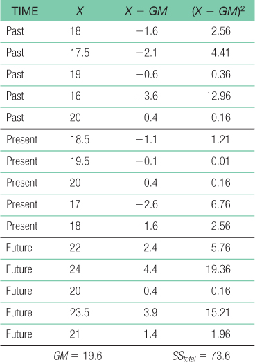
 For sum of squares subjects: SSsubjects = Σ(Mparticipant − GM)2 = 3.429
C-
42 SSwithin = SStotal − SSbetween − SSsubjects = 22.671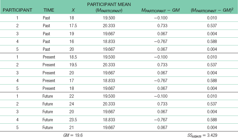 Step 6: The F statistic, 8.38, is beyond 4.46, the critical F value at a p level of 0.05. We would reject the null hypothesis. There is a difference, on average, among the past, present, and future self-
SOURCE SS df MS F Between 47.5 2 23.750 8.38 Subjects 3.429 4 0.857 0.30 Within 22.671 8 2.834 Total 73.6 14 reported life satisfaction of pessimists. - b. First, we calculate sM:
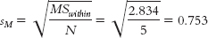
Next, we calculate HSD for each pair of means.
For past versus present: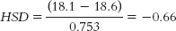
For past versus future: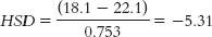
For present versus future: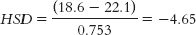
The critical value of q at a p level of 0.05 is 4.04. Thus, we reject the null hypothesis for the past versus future comparison and for the present versus future comparison, but not for the past versus present comparison. These results indicate that the mean self-reported life satisfaction of pessimists is not significantly different for their past and present, but they expect to have greater life satisfaction in the future, on average. - c.
- a. Step 5: We must first calculate df and SS to fill in the source table.
- 13.21dfbetween = Ngroups − 1 = 2
dfsubjects = n − 1 = 4
dfwithin = (dfbetween)(dfsubjects) = 8
dftotal = Ntotal − 1 = 14
For the total sum of squares: SStotal = Σ(X − GM)2 = 4207.335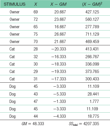 For sum of squares between: SSbetween − Σ(M − GM)2 = 4133.735
C-
43 For sum of squares subjects: SSsubjects = Σ(Mparticipant − GM)2 = 12.675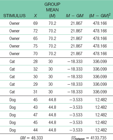 SSwithin = SStotal + SSbetween + SSsubjects = 60.925
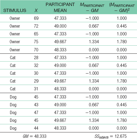
SOURCE SS df MS F Between 4133.735 2 2066.868 271.38 Subjects 12.675 4 3.169 0.42 Within 60.925 8 7.616 Total 4207.335 14 - 13.23 At a p level of 0.05, the critical F value is 4.46. Because the calculated F statistic does not exceed the critical F value, we would fail to reject the null hypothesis. Because we failed to reject the null hypothesis, it would not be appropriate to perform post hoc comparisons.
- 13.25
- a. The independent variable is the type of substance placed beneath the eyes, and its levels are black grease, black antiglare stickers, and petroleum jelly.
- b. The dependent variable is eye glare.
- c. This is a one-
way within- groups ANOVA. - d. The first assumption of ANOVA is that the samples are randomly selected from their populations. It is unlikely that the researchers met this assumption. The study description indicates that the researchers were from Yale University and does not mention any techniques the researchers might have used to obtain participants from across the nation. So it is likely that the Yale researchers used a sample of participants from their local area.
- e. The second assumption is that the population distribution is normal. Although we do not know the exact distribution of the population of scores, there are more than 30 participants in the study. When there are at least 30 participants in a sample, the distribution of sample means will be approximately normal even if the underlying distribution of scores is not. So it is likely that the distribution of sample means is normal and that this assumption was met.
- f. The third assumption is homoscedasticity—
that the samples come from populations with equal variances. Based on the description of the study, it is not possible to tell whether this assumption was met. The researchers could assess whether this assumption was met by comparing the variance of each of the three treatment groups to ensure that the largest variance is no larger than two times the smallest variance. - g. The fourth assumption that is specific to the within-
groups ANOVA is that there are no order effects. To protect against order effects, the researcher would want to have counterbalanced the order in which the participants experienced the treatment conditions. - h. Step 5: We must first calculate df and SS to fill in the source table.
dfbetween = Ngroups − 1 = 2
dfsubjects = n − 1 = 3
dfwithin = (dfbetween)(dfsubjects) = 6
dftotal = Ntotal − 1 = 11For the total sum of squares: SStotal = Σ(X − GM)2 = 16.527C-
44 For the sum of squares between: SSbetween = Σ(M − GM)2 = 13.820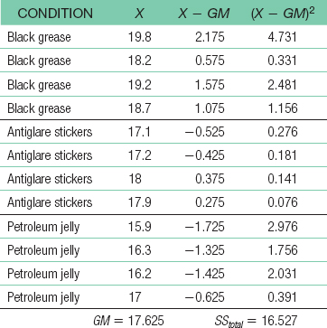 For the sum of squares subjects: SSsubjects = Σ(Mparticipant − GM)2 = 0.735
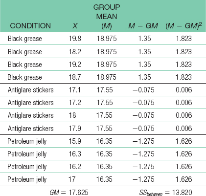 SSwithin = SStotal − SSbetween − SSsubjects = 1.972
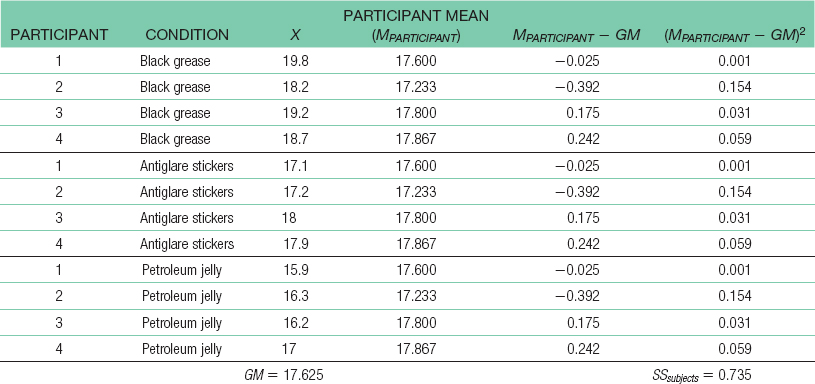
SOURCE SS df MS F Between 13.820 2 6.91 21.00 Subjects 0.735 3 0.245 0.74 Within 1.972 6 0.329 Total 16.527 11 Step 6: The F statistic, 21.00, is beyond 5.14, the critical F value at a p level of 0.05. We would reject the null hypothesis. There is a difference, on average, in the visual acuity of participants while wearing different substances beneath their eyes.C-
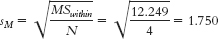
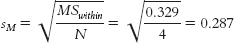
45 - i. First, we calculate sM:
 Next, we calculate HSD for each pair of means.
For grease versus stickers: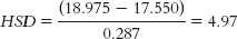
For grease versus jelly: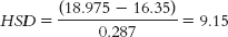
For stickers versus jelly: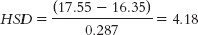
The critical value of q at a p level of 0.05 is 4.34. Thus, we reject the null hypothesis for the grease versus stickers comparison and for the grease versus jelly comparison, but not for the stickers versus jelly comparison. These results indicate that black grease beneath the eyes leads to better visual acuity, on average, than either antiglare stickers or petroleum jelly. - j.
- k. This study could be conducted using a between-
groups design if football players were assigned to only one of the three conditions; thus, they would be exposed to the black grease, the antiglare stickers, or the petroleum jelly, rather than all three. - l. This study could be conducted using a matched-
groups design if the football players in each condition were not the same but were matched based on visual acuity, ability, or other factors we believe may contribute to differences outside the independent variable.