Chapter 18
- 18.1 When we are concerned about meeting the assumptions of a parametric test, we can convert scale data to ordinal data and use a nonparametric test.
- 18.3 When transforming scale data to ordinal data, the scale data are rank ordered. This means that even a very extreme scale score will have a rank that makes it continuous with the rest of the data when rank ordered.
- 18.5 In all correlations, we assess the relative position of a score on one variable with its position on the other variable. In the case of the Spearman rank-
order correlation, we examine how ranks on one variable relate to ranks on the other variable. For example, with a positive correlation, scores that rank low on one variable tend to rank low on the other, and scores that rank high on one variable tend to rank high on the other. For a negative correlation, low ranks on one variable tend to be associated with high ranks on the other. - 18.7 Values for the Spearman rank-
order correlation coefficient range from −1.00 to −1.00, just like they do for its parametric equivalent, the Pearson correlation coefficient. Similarly, the conventions for interpreting the magnitude of the Pearson correlation coefficient can also be applied to the Spearman correlation coefficient (small is roughly 0.10, medium 0.30, and large 0.50). - 18.9 The Wilcoxon signed-
rank test is appropriate to use when comparing two sets of dependent observations (scores from the same participants) and the dependent variable is either ordinal or does not meet the assumptions required by the paired- samples t test. - 18.11 We use absolute values when ranking the differences because what is important is the magnitude of each difference, not its direction. We take into account the directions of the differences when we rank the positive differences versus the negative differences.
- 18.13 The assumptions are that (1) the data are ordinal, (2) random selection was used, and (3) no ranks are tied.
- 18.15 The Kruskal—
Wallis H test is appropriate to use when comparing three or more groups of independent observations (i.e., the independent variable has three or more levels) and the dependent variable is ordinal or does not meet the assumptions of the parametric test. - 18.17 If the data meet the assumptions of the parametric test, then using the parametric test gives us more power to detect a significant effect than does the nonparametric equivalent. Transforming the scale data required for the parametric test into the ordinal data required for the nonparametric test results in a loss of precision of information (i.e., we know that one observation is greater than another, but we don’t know how much greater it is).
- 18.19 Using the bootstrapping method of repeatedly sampling with replacement allows for the estimation of confidence intervals around the original observed sample mean. These confidence intervals can be used to establish likely ranges for the population mean. This method allows the researcher to extrapolate information about population parameters.
- 18.21
- a.
COUNT VARIABLE X RANK X VARIABLE Y RANK Y 1 134.5 3 64.00 7 2 186 10 60.00 1 3 157 9 61.50 2 4 129 1 66.25 10 5 147 7 65.50 8.5 6 133 2 62.00 3.5 7 141 5 62.50 5 8 147 7 62.00 3.5 9 136 4 63.00 6 10 147 7 65.50 8.5 C-
68 - b.
COUNT RANK X RANK Y DIFFERENCE SQUARED DIFFERENCE 1 3 7 −4 16 2 10 1 9 81 3 9 2 7 49 4 1 10 −9 81 5 7 8.5 −1.5 2.25 6 2 3.5 −1.5 2.25 7 5 5 0 0 8 7 3.5 3.5 12.25 9 4 6 −2 4 10 7 8.5 −1.5 2.25 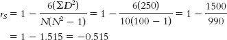
- a.
- 18.23
- a. When calculating the Spearman correlation coefficient, we must first transform the variable “hours trained” into a rank-
ordered variable. We then take the difference between the two ranks and square those differences: We calculate the Spearman correlation coefficient as:RACE RANK HOURS TRAINED HOURS RANK DIFFERENCE SQUARED DIFFERENCE 1 25 1.5 −0.5 0.25 2 25 1.5 0.5 0.25 3 22 3 0 0 4 18 5.5 −1.5 2.25 5 19 4 1 1 6 18 5.5 0.5 0.25 7 12 10 −3 9 8 17 7 1 1 9 15 9 0 0 10 16 8 2 4 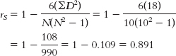
- b. The critical rS with an N of 10, a p level of 0.05, and a two-
tailed test is 0.648. The calculated rS is 0.89, which exceeds the critical value. So we reject the null hypothesis. Finishing place was positively associated with the number of hours spent training.
- a. When calculating the Spearman correlation coefficient, we must first transform the variable “hours trained” into a rank-
- 18.25
- a. To calculate the Wilcoxon signed-
rank test, we first calculate difference scores for each student and then rank those difference scores. Next, we separately sum the ranks associated with the positive and negative difference scores. The sum of the ranks for the positive differences is ΣR+ = 2.0 + 5.5 = 7.5.STUDENT SCHOOL YEAR SUMMER DIFFERENCE RANK RANK FOR POSITIVE DIFFERENCES RANK FOR NEGATIVE DIFFERENCES 1 7 4 3 2.0 2.0 2 4 6 −2 3.5 3.5 3 5 5 0 4 3 4 −1 5.5 5.5 5 4 8 −4 1.0 1.0 6 5 7 −2 3.5 3.5 7 3 2 1 5.5 5.5
The sum of the ranks for the negative differences is ΣR− = 3.5 + 5.5 + 1.0 + 3.5 = 13.5.
T is equal to the smaller of these two sums: T = ΣRsmaller = 7.5. - b. For this data set, N = 6. Although there are 7 participants, there are only 6 nonzero difference scores, and it is the number of nonzero difference scores that determines N for the Wilcoxon signed-
rank test. The critical value for a Wilcoxon signed- rank test with N = 6, a p level of 0.05, and a two- tailed test is 0. Because the calculated T is not smaller than the critical value of 0, we fail to reject the null hypothesis. We do not have evidence that there is a difference between happiness levels during the school year and summer.
C-
69 - a. To calculate the Wilcoxon signed-
- 18.27
The formula for the first group is: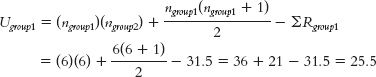
The formula for the second group is: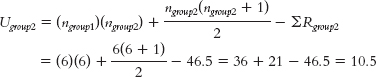
- 18.29
- a. To conduct the Mann—
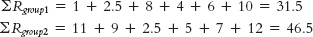
Whitney U test, we first obtain the rank of every person in the data set. We then separately sum the ranks of the two groups, men and women: We sum the ranks for the men: ΣRm = 11 + 3 + 7 + 6 + 8 + 5 = 40.STUDENT GENDER CLASS STANDING RANK MALE RANKS FEMALE RANKS 1 Male 98 11 11 2 Female 72 9 9 3 Male 15 3 3 4 Female 3 1 1 5 Female 102 12 12 6 Female 8 2 2 7 Male 43 7 7 8 Male 33 6 6 9 Female 17 4 4 10 Female 82 10 10 11 Male 63 8 8 12 Male 25 5 5
We sum the ranks for the women: ΣRw = 9 + 1 + 12 + 2 + 4 + 10 = 38.
We calculate U for the men: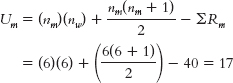
We calculate U for the women: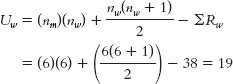
- b. The critical value for the Mann—
Whitney U test with two samples of size 6, a p level of 0.05, and a two- tailed test is 5. We compare the smaller of the two U values to the critical value and reject the null hypothesis if it is smaller than the critical value. Because the smaller U of 17 is not less than 5, we fail to reject the null hypothesis. There is no evidence for a difference in the class standing of men and women.
- a. To conduct the Mann—
- 18.31 To conduct the Kruskal—
Wallis H test, we first rank each participant on the dependent variable and then sort the ranks by group. We then calculate the mean rank for each group (M) and for the whole data set (GM): GROUP SCALE DV RANK GROUP 1 RANK GROUP 2 RANK GROUP 3 RANK Group 1 1.20 7 7 Group 1 1.01 9 9 Group 1 0.86 12 12 Group 1 0.83 13 13 Group 1 0.55 16 16 Group 1 0.22 18 18 Group 2 2.21 4 4 Group 2 1.86 5 5 Group 2 1.03 8 8 Group 2 0.94 10 10 Group 2 0.89 11 11 Group 2 0.74 14 14 Group 3 3.20 1 1 Group 3 2.83 2 2 Group 3 2.75 3 3 Group 3 1.74 6 6 Group 3 0.67 15 15 Group 3 0.52 17 17 Mean rank 9.5 12.5 8.667 7.333 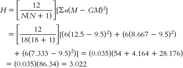
- 18.33
- a. To conduct the Kruskal—
Wallis H test, we first rank each participant on the dependent variable and then sort the ranks by group. We then calculate the mean rank for each group (M) and for the whole data set (GM): GROUP ORDINAL DV RANK GROUP 1 RANK GROUP 2 RANK GROUP 3 RANK Group 1 27 7 7 Group 1 16 9 9 Group 1 15 10 10 Group 2 56 3 3 Group 2 41 4 4 Group 2 38 5 5 Group 2 22 8 8 Group 3 84 1 1 Group 3 72 2 2 Group 3 33 6 6 Group 3 12 11 11 Mean rank 6 8.667 5 5 C-
70 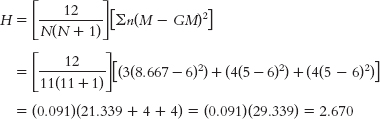
- b. The critical value for the Kruskal—
Wallis H test is found using the table for chi square. The df is the number of groups minus 1, which in this case is 2. For df = 2, a p level of 0.05, and a two- tailed test, the critical value is 5.992. We fail to reject the null hypothesis because the calculated H does not exceed this critical value.
- a. To conduct the Kruskal—
- 18.35
- a. The Mann—
Whitney U test would be most appropriate because it is a nonparametric equivalent to the independent- samples t test. It is used when there is a nominal independent variable with two levels (north and south of the equator), a between- groups research design, and an ordinal dependent variable (the ranking of the city). - b. The Wilcoxon signed-
rank test would be most appropriate because there is a nominal independent variable with two levels (the time of the previous study versus 2012), a within- groups research design, and an ordinal dependent variable (ranking). The Wilcoxon signed- rank test is the nonparametric equivalent to the paired- samples t test. - c. The Spearman rank-
order correlation would be most appropriate because this is a question about the relation between two ordinal variables. The Spearman rank- order correlation is the nonparametric equivalent to the Pearson correlation. - d. The Kruskal-
Wallis H test would be most appropriate because it is a nonparametric equivalent to the one- way between- groups ANOVA. It is used when there is a nominal independent variable with three or more levels (the various continents, in this case), a between- groups research design, and an ordinal dependent variable (the ranking of the city).
- a. The Mann—
- 18.37
- a. The first variable of interest is test grade, which is a scale variable. The second variable of interest is the order in which students completed the test, which is an ordinal variable.
- b. The accompanying table shows test grade converted to ranks, difference scores, and squared differences.We calculate the Spearman correlation coefficient as:
GRADE PERCENTAGE GRADE SPEED RANK D D2 98 1 1 0 0 93 6 2 4 16 92 4 3 1 1 88 5 4 1 1 87 3 5 −2 4 74 2 6 −4 16 67 8 7 1 1 62 7 8 −1 1 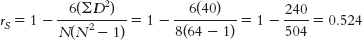
- c. The coefficient tells us that there is a rather large positive relation between the two variables. Students who completed the test more quickly also tended to score higher.
- d. We could not have calculated a Pearson correlation coefficient because one of the variables, order in which students turned in the test, is ordinal.
- e. This correlation does not indicate that students should attempt to take their tests as quickly as possible. Correlation does not provide evidence for a particular causal relation. A number of underlying causal relations could produce this observed correlation.
- f. A third variable that might cause both speedy test taking and a good test grade is knowledge of the material. Students with better knowledge of, and more practice with, the material would be able to get through the test more quickly and get a better grade.
- f. The coefficient of 0.09 indicates a small positive relation between the two variables. There is a small tendency for students who turn their exams in earlier to get better grades.
- 18.39
- a. The independent variable is the season, and its levels are 1995–
1996 and 2005– 2006. The dependent variable is the number of wins per season. - b. This is a within-
groups design because the same teams are being assessed at two different time points. - c. It would be preferable to conduct a nonparametric test because there is a very small sample size and the dependent variable, number of wins, is not likely to be normally distributed in the population.
- d. Step 1: We will convert the scale data into ordinal data. It is difficult to know from this small sample whether the difference scores come from a symmetric population distribution. (Note: These were all of the Canadian NHL teams that existed in those two seasons, so the assumption of random selection is irrelevant.)
Step 2: Null hypothesis: There is no difference between the teams’ performance rankings in the 1995–1996 season and those in the 2005– 2006 season.
Research hypothesis: There is a difference between the teams’ performance rankings in the 1995–1996 season and those in the 2005– 2006 season.
Step 3: The comparison distribution will be a T distribution. We will use a p level of 0.05 and a two-tailed test. The sample size is 6.
Step 4: The critical T value is 0. The calculated T value must be less than or equal to 0 to be statistically significant.Step 5: (Note: The difference scores are positive because they reflect an increase in wins.)C-
71 TEAM 1995– 1996 SEASON 2005– 2006 SEASON D D RANK POSITIVE DIFFERENCE NEGATIVE DIFFERENCE Calgary Flames 34 46 12 2 2 Edmonton Oilers 30 41 11 3 3 Montréal Canadiens 40 42 2 6 6 Ottawa Senators 18 52 34 1 1 Toronto Maple Leafs 34 41 7 5 5 Vancouver Canucks 32 42 10 4 4 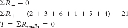
Step 6: The test statistic, 0, is equal to the critical value, so we reject the null hypothesis. Canadian teams had more wins in the 2005–2006 season than in the 1995– 1996 season. - e. T = 0, p = 0.05
- a. The independent variable is the season, and its levels are 1995–
- 18.41
- a. The independent variable is the type of institution and its levels are public and private. The dependent variable is U.S. News & World Report ranking.
- b. This is a between-
groups design because the institutions are either public or private but cannot be both. - c. We have to use a nonparametric test for these data because the dependent measure is ordinal.
- d. Step 1: The data are ordinal. The schools on the list have not been randomly selected but were systematically selected (they are the top 19 programs in the United States). Finally, a number of schools have tied ranks. The results of the Mann—
Whitney U test may not be valid.
Step 2: Null hypothesis: There will tend to be no difference between the rankings of public and private schools.
Research hypothesis: There will tend to be a difference between the rankings of public and private schools.
Step 3: There are 9 public universities and 10 private universities listed.
Step 4: The critical value for a Mann—Whitney U test with one group of 9 and one group of 10, a p level of 0.05, and a two- tailed test is 20. The calculated statistic will need to be less than or equal to this critical value to be considered statistically significant.
Step 5:UNIVERSITY RANK TYPE OF SCHOOL PUBLIC RANK PRIVATE RANK Princeton University 2 Private 2 University of California, Berkeley 2 Public 2 University of Wisconsin, Madison 2 Public 2 Stanford University 4.5 Private 4.5 University of Michigan, Ann Arbor 4.5 Public 4.5 Harvard University 7 Private 7 University of Chicago 7 Private 7 University of North Carolina, Chapel Hill 7 Public 7 University of California, Los Angeles 9 Public 9 Northwestern University 10.5 Private 10.5 University of Pennsylvania 10.5 Private 10.5 Columbia University 12.5 Private 12.5 Indiana University, Bloomington 12.5 Public 12.5 Duke University 14.5 Private 14.5 University of Texas, Austin 14.5 Public 14.5 New York University 16 Private 16 Cornell University 18 Private 18 Ohio State University 18 Public 18 Pennsylvania State University, University Park 18 Public 18 C-
72 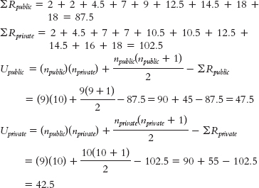
Step 6: The smaller U statistic, 42.5, is not smaller than the critical value of 20, so we fail to reject the null hypothesis. - e. U = 42.5, p > 0.05
- 18.43
- a. Hours studied per week appears to be roughly normal, with observations across the range of values—
from 0 through 20. Monthly cell phone bill appears to be positively skewed, with one observation much higher than all the others. - b. The histogram confirms the impression that the monthly cell phone bill is positively skewed. It appears that there is an outlier in the distribution.
- c. Parametric tests assume that the underlying population data are normally distributed or that there is a large enough sample size that the sampling distribution will be normal anyway. These data seem to indicate that the underlying distribution is not normally distributed; moreover, there is a fairly small sample size (N = 29). We would not want to use a parametric test.
- a. Hours studied per week appears to be roughly normal, with observations across the range of values—
- 18.45
- a. The independent variable is region of the country, and its levels are Northeast, Midwest, and South. The dependent variable is “smart” ranking.
- b. This is a between-
groups design because a state is in only one region of the country. - c. We need to use a nonparametric test because the dependent measure is ordinal.
- d. Step 1: The data are ordinal. (This list includes all states in the regions of interest, so the assumption of random selection is not relevant.)
Step 2: Null hypothesis: The “smart” ranking of a state does not tend to vary with the state’s geographical region. Research hypothesis: The “smart” ranking of a state does tend to vary with the state’s geographical region.
Step 3: We will use the chi-square distribution as the comparison distribution with degrees of freedom of 3 − 1 = 2.
Step 4: The critical value with a df of 2 and p level of 0.05 is 5.992. The calculated statistic will need to be larger than this critical value to be considered statistically significant.
Step 5:STATE RANK NE RANK MW RANK S RANK Massachusetts 1 1 Connecticut 2 2 Vermont 3 3 New Jersey 4 4 Wisconsin 5 5 New York 6 6 Minnesota 7 7 Iowa 8 8 Pennsylvania 9 9 Maine 10 10 Virginia 11 11 Nebraska 12 12 New Hampshire 13 13 Kansas 14 14 Indiana 15 15 Ohio 16 16 Rhode Island 17 17 Illinois 18 18 North Carolina 19 19 Missouri 20 20 Michigan 21 21 South Carolina 22 22 Arkansas 23 23 Kentucky 24 24 Georgia 25 25 Florida 26 26 Tennessee 27 27 Alabama 28 28 Louisiana 29 29 Mississippi 30 30 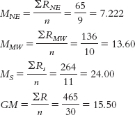
C-
73 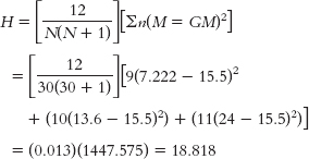
Step 6: The calculated statistic, 18.818, exceeds the critical value of 5.992, so we reject the null hypothesis. The “smart” ranking for a state does tend to vary with the geographical location of that state. - e. H = 18.82, p < 0.05
- f. Like a one-
way between- groups ANOVA, the Kruskal— Wallis H statistic when used with more than two groups just indicates that there is a difference among the groups, but it does not indicate where that difference is. Separate Kruskal— Wallis H tests for each group comparison in the current example appear below. For each test, the df is 1 and the critical value, given a p level of 0.05, is 3.84.
Northeast versus South: H = 13.02, p < 0.05
Northeast versus Midwest: H = 4.86, p < 0.05
Midwest versus South: H = 10.49, p < 0.05
All regions are statistically significantly different from each other. The states in the Northeast tend to have the highest rankings, followed by those in the Midwest, and then by those in the South. - g. If there were scale scores for the 50 states, we could conduct a parametric test—
specifically a one- way between- groups ANOVA— to determine differences among the three levels, or groups, of states. - h. Intelligence could be operationally defined as the state average on IQ or other intelligence tests, or in the percentage of people with various levels of education.
C-
74