Chapter 6
- 6.1 In everyday conversation, the word normal is used to refer to events or objects that are common or that typically occur. Statisticians use the word to refer to distributions that conform to a specific bell-
shaped curve, with a peak in the middle where most of the observations lie, and symmetric areas underneath the curve on either side of the midpoint. This normal curve represents the pattern of occurrence of many different kinds of events. - 6.3 The distribution of sample scores approaches normal as the sample size increases, assuming the population is normally distributed.
- 6.5 A z score is a way to standardize data; it expresses how far a data point is from the mean of its distribution in terms of standard deviations.
- 6.7 The mean is 0 and the standard deviation is 1.0.
- 6.9 The symbol μM stands for the mean of the distribution of means. The μ indicates that it is the mean of a population, and the subscript M indicates that the population is composed of sample means—the means of all possible samples of a given size from a particular population of individual scores.
- 6.11 Standard deviation is the measure of spread for a distribution of scores in a single sample or in a population of scores. Standard error is the standard deviation (or measure of spread) in a distribution of means of all possible samples of a given size from a particular population of individual scores.
- 6.13 The z statistic tells us how many standard errors a sample mean is from the population mean.
- 6.15
- a.
- b.
- c.
- d. As the sample size increases, the distribution approaches the shape of the normal curve.
C-
16 - a.
- 6.17
- a.
- b.
- c.
- d.
- a.
- 6.19
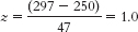
Each of these scores is 47 points away from the mean, which is the value of the standard deviation. The z scores of +1.0 and 1.0 express that the first score, 203, is 1 standard deviation below the mean, whereas the other score, 297, is 1 standard deviation above the mean. - 6.21
- a. X = z(σ) + μ = −0.23(164) + 1179 = 1141.28
- b. X = 1.41(164) + 1179 = 1410.24
- c. X = 2.06(164) + 1179 = 1516.84
- d. X = 0.03(164) + 1179 = 1183.92
- 6.23
- a. X = z(σ) + μ = 1.5(100) + 500 = 650
- b. X = z(σ) + μ = −0.5(100) + 500 = 450
- c. X = z(σ) + μ = −2.0(100) + 500 = 300
- 6.25
- a.
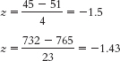
- b. Both of these scores fall below the means of their distributions, resulting in negative z scores. One score (45) is a little farther below its mean than the other (732).
- a.
- 6.27
- a. 50%
- b. 82% (34 + 34 + 14)
- c. 4% (2 + 2)
- d. 48% (34 + 14)
- e. 100% or nearly 100%
- 6.29
- a.
- b.
- c.
- a.
- 6.31
- a.
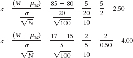
- b. The first sample had a mean that was 2.50 standard deviations above the population mean, whereas the second sample had a mean that was 4 standard deviations above the mean. Compared to the population mean (as measured by this scale), both samples are extreme scores; however, a z score of 4.0 is even more extreme than a z score of 2.5.
- a.
- 6.33
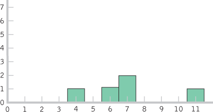
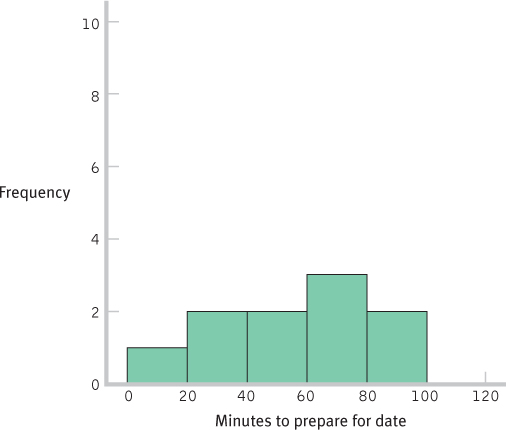
- a. Histogram for the 10 scores:
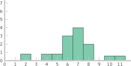
- b. Histogram for the 40 scores:
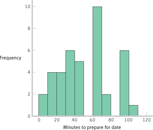
- c. The shape of the distribution became more normal as the number of scores increased. If we added more scores, the distribution would become more and more normal. This happens because many physical, psychological, and behavioral variables are normally distributed. With smaller samples, this might not be clear. But as the sample size approaches the size of the population, the shape of the sample distribution approaches that of the population.
- d. These are distributions of scores, as each individual score is represented in the histograms on its own, not as part of a mean.
C-
17 - e. There are several possible answers to this question. For example, instead of using retrospective self-
reports, we could have had students call a number or send an e- mail as they began to get ready; they would then have called the same number or sent another e- mail when they were ready. This would have led to scores that would be closer to the actual time it took the students to get ready. - f. There are several possible answers to this question. For example, we could examine whether there was a mean gender difference in time spent getting ready for a date.
- a. Histogram for the 10 scores:
- 6.35
- a. The mean of the z distribution is always 0.
- b.
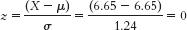
- c. The standard deviation of the z distribution is always 1.
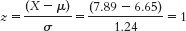
- d. A student 1 standard deviation above the mean would have a score of 6.65 + 1.24 = 7.89. This person’s z score would be:
- e. The answer will differ for each student but will involve substituting one’s own score for X in this equation:

- 6.37
- a. It would not make sense to compare the mean of this sample to the distribution of individual scores because, in a sample of means, the occasional extreme individual score is balanced by less extreme scores that are also part of the sample. Thus, there is less variability.
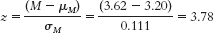
- b. The null hypothesis would state that the population from which the sample was drawn has a mean of 3.20. The research hypothesis would state that the mean for the population from which our sample was drawn is not 3.20.
- c.
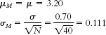
- d.
- 6.39
- a. Yes, the distribution of the number of movies college students watch in a year would likely approximate a normal curve. You can imagine that a small number of students watch an enormous number of movies and that a small number watch very few but that most watch a moderate number of movies between these two extremes.
- b. Yes, the number of full-
page advertisements in magazines is likely to approximate a normal curve. We could find magazines that have no or just one or two full- page advertisements and some that are chock full of them, but most magazines have some intermediate number of full- page advertisements. - c. Yes, human birth weights in Canada could be expected to approximate a normal curve. Few infants would weigh in at the extremes of very light or very heavy, and the weight of most infants would cluster around some intermediate value.
- 6.41
- a.
- b.
- c. According to these data, the Falcons had a better regular season (they had a higher z score) than did the Braves.
- d. The Braves would have had to have won 101 regular season games to have a slightly higher z score than the Falcons:
- e. There are several possible answers to this question. For example, we could have summed the teams’ scores for every game (as compared to other teams∈ scores within their leagues).
- a.
- 6.43
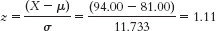
- a. X = z(σ) + μ = −1.705(11.733) + 81.00 = 61 games (rounded to a whole number)
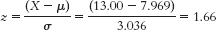
- b. X = (σ) + μ = −0.319(3.036) + 7.969 = 7 games (rounded to a whole number)
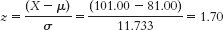
- c. Fifty percent of scores fall below the mean, so 34% (84 − 50 = 34) fall between the mean and the Colts’ score. We know that 34% of scores fall between the mean and a z score of 1.0, so the Colts have a z score of 1.0. X = z(σ) + μ = 1(3.036) + 7.969 = 11 games (rounded to a whole number).
- d. We can examine our answers to be sure that negative z scores match up with answers that are below the mean and positive z scores match up with answers that are above the mean.
- 6.45
- a. μ = 50; σ = 10
- b.
- c. When we calculate the mean of the scores for 95 individuals, the most extreme MMPI-
2 depression scores will likely be balanced by scores toward the middle. It would be rare to have an extreme mean of the scores for 95 individuals. Thus, the spread is smaller than is the spread for all of the individual MMPI- 2 depression scores.
- 6.47
- a. These are the data for a distribution of scores rather than means because they have been obtained by entering each individual score into the analysis.
- b. Comparing the sizes of the mean and the standard deviation suggests that there is positive skew. A person can’t have fewer than zero friends, so the distribution would have to extend in a positive direction to have a standard deviation larger than the mean.
- c. Because the mean is larger than either the median or the mode, it suggests that the distribution is positively skewed. There are extreme scores in the positive end of the distribution that are causing the mean to be more extreme than the median or mode.
- d. You would compare this person to the distribution of scores. When making a comparison of an individual score, we must use the distribution of scores.
- e. You would compare this sample to a distribution of means. When making a comparison involving a sample mean, we must use a distribution of means because it has a different pattern of variability from a distribution of scores (it has less variability).
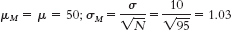
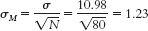
- f. μM = μ = 7.44. The number of individuals in the sample is 80. Substituting 80 in the standard error equation yields
C-
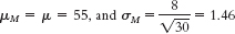
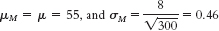
18 - g. The distribution of means is likely to be a normal curve. Because the sample of 80 is well above the 30 recommended to see the central limit theorem at work, we expect that the distribution of the sample means will approximate a normal distribution.
- 6.49
- a. You would compare this sample mean to a distribution of means. When we are making a comparison involving a sample mean, we need to use the distribution of means because it is this distribution that indicates the variability we are likely to see in sample means.
- b.
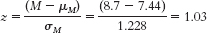
This z statistic of 1.03 is approximately 1 standard deviation above the mean. Because 50% of the sample are below the mean and 34% are between the mean and 1 standard deviation above it, this sample would be at approximately the 84th percentile. - c. It does make sense to calculate a percentile for this sample. Given the central limit theorem and the size of the sample used to calculate the mean (80), we would expect the distribution of the sample means to be approximately normal.
- 6.51
- a. The population is all patients treated for blocked coronary arteries in the United States. The sample is Medicare patients in Elyria, Ohio, who received angioplasty.
- b. Medicare and the commercial insurer compared the angioplasty rate in Elyria to that in other towns. Given that the rate was so far above that of other towns, they decided that such a high angioplasty rate was unlikely to happen just by chance. Thus, they used probability to make a decision to investigate.
- c. Medicare and the commercial insurer could look at the z distribution of angioplasty rates in cities from all over the country. Locating the rate of Elyria within that distribution would indicate exactly how extreme or unlikely its angioplasty rates are.
- d. The error made would be a Type I error, as they would be rejecting the null hypothesis that there is no difference among the various towns in rates of angioplasty, and concluding that there is a difference, when there really is no difference.
- e. Elyria’s extremely high rates do not necessarily mean the doctors are committing fraud. One could imagine that an area with a population composed mostly of retirees (that is, more elderly people) would have a higher rate of angioplasty. Conversely, perhaps Elyria has a talented set of surgeons who are renowned for their angioplasty skills and people from all over the country come there to have angioplasty.
- 6.53
- a. The researchers are operationally defining cheating as the change in standardized test score for a given classroom. This variable is a scale variable.
- b. Researchers could establish a cut-
off z statistic at which those who had a mean change larger than that z statistic would be considered “suspicious.” For example, a classroom with a z statistic of 2 or more may have cheated on this year’s test. - c. A histogram or frequency polygon would provide an easy visual to see where a given classroom falls on the distribution. A researcher could even draw lines indicating the cutoffs and see which classrooms fall beyond them.
- d. They would be committing a Type I error, because they would be rejecting the null hypothesis that there is no difference in a classroom’s test scores from one year to the next when there really is no difference and they should have failed to reject the null hypothesis.