Chapter 7
- 7.1 A percentile is the percentage of scores that fall below a certain point on a distribution.
- 7.3 We add the percentage between the mean and the positive z score to 50%, which is the percentage of scores below the mean (50% of scores are on each side of the mean).
- 7.5 In statistics, assumptions are the characteristics we ideally require the population from which we are sampling to have so that we can make accurate inferences.
- 7.7Parametric tests are statistical analyses based on a set of assumptions about the population. By contrast, nonparametric tests are statistical analyses that are not based on assumptions about the population.
- 7.9Critical values, often simply called cutoffs, are the test statistic values beyond which we reject the null hypothesis. The critical region refers to the area in the tails of the distribution in which the null hypothesis will be rejected if the test statistic falls there.
- 7.11 A statistically significant finding is one in which we have rejected the null hypothesis because the pattern in the data differed from what we would expect by chance. The word significant has a particular meaning in statistics. “Statistical significance” does not mean that the finding is necessarily important or meaningful. Statistical significance only means that we are justified in believing that the pattern in the data is likely to reoccur; that is, the pattern is likely genuine.
- 7.13Critical region may have been chosen because values of a test statistic describe the area beneath the normal curve that represents a statistically significant result.
- 7.15 For a one-
tailed test, the critical region (usually 5%, or a p level of 0.05) is placed in only one tail of the distribution; for a two- tailed test, the critical region must be split in half and shared between both tails (usually 2.5%, or 0.025, in each tail). - 7.17 The following are the two options for one-
tailed test hypotheses. - 1) Null hypothesis: H0: μ1 ≥ μ2
Research hypothesis: H1: μ1 < μ2 - 2) Null hypothesis: H0: μ1 ≥ μ1
Research hypothesis: H1: μ1 > μ2
- 1) Null hypothesis: H0: μ1 ≥ μ2
- 7.19
- (1) Replace the missing data point with the mode or mean for that variable (based on other participants’ responses).
- (2) Replace the missing data point with the mode or mean based on that participant’s responses to other, similar questions.
- (3) Replace the missing data point with a random number within the possible range of numbers.
C-
19 - 7.21
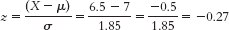
- a. If 22.96% are beyond this z score (in the tail), then 77.04% are below it (100% − 22.96%).
- b. If 22.96% are beyond this z score, then 27.04% are between it and the mean (50% − 22.96%).
- c. Because the curve is symmetric, the area beyond a z score of − 0.74 is the same as that beyond 0.74. Expressed as a proportion, 22.96% appears as 0.2296.
- 7.23
- a. The percentage above is the percentage in the tail, 4.36%.
- b. The percentage below is calculated by adding the area below the mean, 50%, and the area between the mean and this z score, 45.64%, to get 95.64%.
- c. The percentage at least as extreme is computed by doubling the amount beyond the z score, 4.36%, to get 8.72%.
- 7.25
- a. 19%
- b. 4%
- c. 92%
- 7.27
- a. 2.5% in each tail
- b. 5% in each tail
- c. 0.5% in each tail
- 7.29μM = μ = 500
- 7.31
- a. Fail to reject the null hypothesis because 1.06 does not exceed the cutoff of 1.96.
- b. Reject the null hypothesis because −2.06 is more extreme than −1.96.
- c. Fail to reject the null hypothesis because a z statistic with 7% of the data in the tail occurs between ±1.48 and ±1.47, which are not more extreme than ±1.96.
- 7.33
- a. Fail to reject the null hypothesis because 0.95 does not exceed 1.65.
- b. Reject the null hypothesis because −1.77 is more extreme than −1.65.
- c. Reject the null hypothesis because the critical value resulting in 2% in the tail falls within the 5% cutoff region in each tail.
- 7.35
- a. The situation describes misleading data. Given that the participant’s responses did not vary at all, it is likely that he or she either did not read the statements or did not take the survey seriously.
- b. The situation does not describe misleading data. The participant’s response time of 420 ms is a likely response given the sample mean of 413 ms and standard deviation of 30 ms.
- c. The situation describes misleading data. Given the mean and standard deviation she found in previous studies, this observation of 1220 is unlikely (perhaps the participant sneezed—
or dozed off).
- 7.37
- a.
The percentage below is 19.49%. - b.
The percentage below is 50% + 29.10% = 79.10%. - c.
The percentage below is 50% + 34.85% = 84.85%. - d.
The percentage below is 39.36%.
- a.
- 7.39
- a.
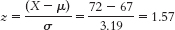
- b. 44.18% of scores are between this z score and the mean. We need to add this to the area below the mean, 50%, to get the percentile score of 94.18%.
- c. 94.18% of boys are shorter than Kona at this age.
- d. If 94.18% of boys are shorter than Kona, that leaves 5.82% in the tail. To compute how many scores are at least as extreme, we double this to get 11.64%.
- e. We look at the z table to find a critical value that puts 30% of scores in the tail, or as close as we can get to 30%. A
z score of −0.52 puts 30.15% in the tail. We can use that z score to compute the raw score for height:
X = −0.52(3.19) + 67 = 65.34 inches
At 72 inches tall, Kona is 6.66 inches taller than Ian.
- a.
- 7.41
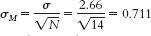
- a.
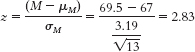
- b. The z statistic indicates that this sample mean is 2.83 standard deviations above the expected mean for samples of size 13. In other words, this sample of boys is, on average, exceptionally tall.
- c. The percentile rank is 99.77%, meaning that 99.77% of sample means would be of lesser value than the one obtained for this sample.
- a.
- 7.43
- a. μM = μ = 63.8
- b.
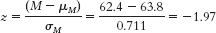
- c. 2.44% of sample means would be shorter than this mean.
- d. We double 2.44% to account for both tails, so we get 4.88% of the time.
- e. The average height of this group of 15-
year- old females is rare, or statistically significant.
- a. μM = μ = 63.8
- 7.45
- a. This is a nondirectional hypothesis because the researcher is predicting that it will alter skin moisture, not just decrease it or increase it.
- b. This is a directional hypothesis because better grades are expected.
- c. This hypothesis is nondirectional because any change is of interest, not just a decrease or an increase in closeness of relationships.
C-
20 - 7.47
- a.
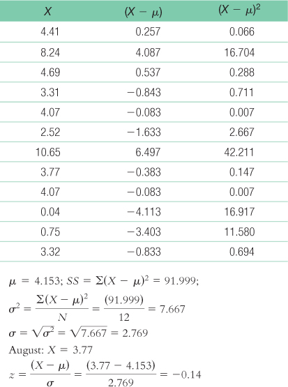
- b. The table tells us that 44.43% of scores fall in the tail beyond a z score of − 0.14. So, the percentile for August is 44.43%. This is surprising because it is below the mean, and it was the month in which a devastating hurricane hit New Orleans. (Note: It is helpful to draw a picture of the curve when calculating this answer.)
- c. Paragraphs will be different for each student but will include the fact that a monthly total based on missing data is inaccurate. The mean and the standard deviation based on this population, therefore, are inaccurate. Moreover, even if we had these data points, they would likely be large and would increase the total precipitation for August; August would likely be an outlier, skewing the overall mean. The median would be a more accurate measure of central tendency than the mean under these circumstances.
- d. We would look up the z score that has 10% in the tail. The closest z score is 1.28, so the cutoffs are − 1.28 and 1.28. (Note: It is helpful to draw a picture of the curve that includes these z scores.) We can then convert these z scores to raw scores. X = z(σ) + μ = −1.28(2.769) + 4.153 = 0.61; X = z(σ) + μ = 1.28(2.769) + 4.153 = 7.70. Only October (0.04) is below 0.61. Only February (8.24) and July (10.65) are above 7.70. These data are likely inaccurate, however, because the mean and the standard deviation of the population are based on an inaccurate mean from August. Moreover, it is quite likely that August would have been in the most extreme upper 10% if there were complete data for this month.
- a.
- 7.49
- a. Population 1 is adult psychiatric inpatients. Population 2 is adult nonpatients.
- b. The comparison distribution would be a distribution of means. Boone would compare his sample of 150 psychiatric inpatients to a distribution of the means of all possible samples of 150 individuals.
- c. You would use a z test because there is one sample and you are comparing it to a population for which you know the mean and the standard deviation.
- d. (1) From the description, the dependent variable—
intrasubtest scatter— seems to be a scale variable. (2) The sample includes 150 adult psychiatric inpatients. It is unlikely that they were randomly selected from all adult psychiatric inpatients; thus, we must be cautious about generalizing from this sample. (3) We do not know if the population distribution is normal, but we have more than 30 participants (to be specific, we have 150), so the sampling distribution is likely to be normal. - e. Boone uses the word significantly as an indication that he rejected the null hypothesis.
- 7.51
- a. The independent variable is the division. Teams were drawn from either the Football Bowl Subdivision (FBS) or the Football Championship Division (FCS). The dependent variable is the spread.
- b. Random selection was not used. Random selection would entail having some process for randomly selecting FCS games for inclusion in the sample. We did not describe such a process and, in fact, took all the FCS teams from one league within that division.
- c. The populations of interest are football games between teams in the upper divisions of the NCAA (FBS and FCS).
- d. The comparison distribution would be the distribution of sample means.
- e. The first assumption—
that the dependent variable is a scale variable— is met in this example. The dependent variable is point spread, which is a scale measure. The second assumption— that participants are randomly selected— is not met. As described in part (b), the teams for inclusion in the sample were not randomly selected. The third assumption— that the distribution of scores in the population of interest must be normal— is not likely to have been met. The standard deviation is almost as large as the mean, an indication that one or more outliers are creating positive skew. Moreover, we only have a sample size of 4, not the 30 we would need to have a normal distribution of means.
- 7.53
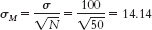
- a. Step 3: μM = μ = 16.189;
Step 4: When we adopt 0.05 as the p level for significance and have a two-tailed hypothesis, we need to divide the 0.05 by 2 to obtain the z score cutoff for each end of the distribution (high and low). Dividing 0.05 by 2 yields 0.025. The z score corresponding to a probability of 0.025 is 1.96. Therefore, the cutoffs are −1.96 and 1.96.
Step 5: We first must obtain the mean spread in the sample. The games and their spreads are listed here:GAME SPREAD Holy Cross, 27/Bucknell, 10 17 Lehigh, 23/Colgate, 15 8 Lafayette, 31/Fordham, 24 7 Georgetown, 24/Marist, 21 3 Mean spread = 8.75C-
21 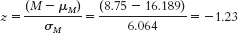
Step 6: Given that the z statistic of −1.23 is not beyond the cutoff of −1.96, we would fail to reject the null hypothesis. We can conclude only that we do not have sufficient evidence that the point spread of FCS teams is different, on average, from that of FBS teams. - b. It would be unwise to generalize these findings beyond the sample. The sample of games was not randomly selected from all FCS team games that week. It is possible that this particular league differs from other leagues and therefore is not representative of the FCS as a whole.
- a. Step 3: μM = μ = 16.189;
- 7.55
- a. The independent variable is whether a patient received the DVD with information about orthodontics. One group received the DVD; the other group did not. The dependent variable is the number of hours per day patients wore their appliances.
- b. The researcher did not use random selection when choosing his sample. He selected the next 15 patients to come into his clinic.
- c. Step 1: Population 1 is patients who did not receive the DVD. Population 2 is patients who received the DVD. The comparison distribution will be a distribution of means. The hypothesis test will be a z test because we have only one sample and we know the population mean and the standard deviation. This study meets the assumption that the dependent variable is a scale measure. We might expect the distribution of number of hours per day people wear their appliances to be normally distributed, but from the information provided it is not possible to tell for sure. Additionally, the sample includes fewer than 30 participants, so the central limit theorem may not apply here. The distribution of sample means may not approach normality. Finally, the participants were not randomly selected. Therefore, we may not want to generalize the results beyond this sample.
Step 2: Null hypothesis: Patients who received the DVD do not wear their appliances a different mean number of hours per day than patients who did not receive the DVD; H0: μ1 = μ2.
Research hypothesis: Patients who received the DVD wear their appliances a different mean number of hours per day than patients who did not receive the DVD; H1: μ1 ≠ μ2.
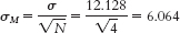
Step 3: μM = μ = 14.78;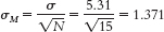
Step 4: The cutoff z statistics, based on a p level of 0.05 and a two-tailed test, are −1.96 and 1.96. (Note: It is helpful to draw a picture of the normal curve and include these z statistics on it.)
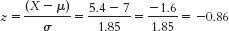
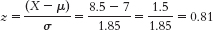
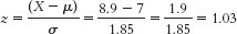
Step 5: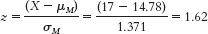
(Note: It is helpful to add this z statistic to your drawing of the normal curve that includes the cutoff z statistics.)
Step 6: Fail to reject the null hypothesis. We cannot conclude that receiving the DVD improves average patient compliance. - d. The researcher would have made a Type II error. He would have failed to reject the null hypothesis when a mean difference actually existed between the two populations.
- 7.57
- a. There are several possible causes of the incomplete data on the sexual behavior scale. One potential cause is that participants were unwilling to share information about certain aspects of their life, particularly their sexual behavior. A second possible cause is that participants became fatigued or bored partway through working on the scales. A third possible cause is that the participants were unmotivated to complete the scales.
- b. There are several options for dealing with the missing data on the sexual behavior scale if only 1 or 2 answers are missing. First, you could replace missing values for a participant with the modal or mean score for all participants on that variable. Second, you could replace the missing values for a participant with that participant’s modal or mean score on similar items on the scale. Finally, you could replace the missing values for a participant with a random number within the range of possible responses. We would exclude from the study people who completed none or only half the items.
- c. You might decide to exclude the participant who had the highest possible scores on every item on both scales (and finished very quickly) from your analysis. You would, however, need to report that you did so when you write up your results.
- d. You should report all of your decisions for handling missing data and outliers when you write up your results. The primary test of whether a result is real is whether it can be replicated. You want other researchers to be able to replicate your work. To do so, they need to know precisely how you handled your data. Furthermore, to advance science, you need to be honest about difficulties you encountered. That way, future researchers can either expect to have the same difficulties or can attempt to improve on your methodology to avoid those difficulties.
- 7.59
- a. The data from Marvel’s The Avengers ($1512 million) and Skyfall ($1109 million) seem to be outliers, as they are the only scores close to or above $1,000,000 (represented by a score over 1000 in the table in the exercise). Life of Pi ($609 million) also appears to be much higher than the other scores, which range from $59 to $397 million.
- b.
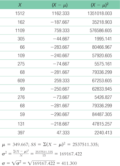 The raw score for a z score of −2.00 is X = z(σ) + μ = −2.00(411.300) + 349.667 = −472.93. This number doesn’t make sense here as there are no movies listed that lost $473 million. Thus, there are no outliers below a z score of −2.00.
C-
22
The raw score for a z score of 2.00 is X = z(σ) + μ = 2.00(411.300) + 349.667 = 1172.27. The only movie that made more than this value of $1,172,270 was Marvel’s The Avengers, which made $1,512,000. Thus, this is the only outlier in the data. - c. The raw score for a z score of −3.00 is X = z(σ) + μ = −3.00(411.300) + 349.667 = −884.23. Like in part (b), this number doesn’t make sense here as there are no movies listed that lost $884 million. Thus, there are no outliers below a z score of −3.00.
The raw score for a z score of 3.00 is X = z(σ) + μ = 3.00(411.300) + 349.667 = 1583.57. Though one movie was determined to be an outlier in part (b), according to this standard of 3 standard deviations above the mean, it is no longer considered an outlier since $1,512,000 is less than $1,583,000. Thus, there are no outliers in the data using this standard. - d. Outliers are extreme scores that skew the data, especially in calculating the mean and standard deviation. They also demonstrate scores that are not representative of the typical scores one would obtain. Eliminating outliers allows us to more accurately calculate measures of central tendency and variability, as well as identify scores that are more typical of the population. However, it is important to evaluate why the outlier may have occurred and what it tells us about the data or data collection process.
- e. In order to eliminate biases the researcher may have regarding what should or should not be included in the data after viewing the results, the researcher should prepare methods for dealing with outliers before collecting data. Much like generating hypotheses before the study begins, preparing methods to deal with outliers or other data issues allow us to be more objective in analyzing the data.