nolanheinzen3e

Chapter 8

8.1 There may be a statistically significant difference between group means, but the difference might not be meaningful or have a real-life application.
8.3 Confidence intervals add details to the hypothesis test. Specifically, they tell us a range within which the population mean would fall 95% of the time if we were to conduct repeated hypothesis tests using samples of the same size from the same population.
8.5 In everyday language, we use the word effect to refer to the outcome of some event. Statisticians use the word in a similar way when they look at effect sizes. They want to assess a given outcome. For statisticians, the outcome is any change in a dependent variable, and the event creating the outcome is an independent variable. When statisticians calculate an effect size, they are calculating the size of an outcome.
8.7 If two distributions overlap a lot, then we would probably find a small effect size and not be willing to conclude that the distributions are necessarily different. If the distributions do not overlap much, this would be evidence for a larger effect or a meaningful difference between them.
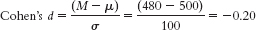
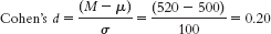
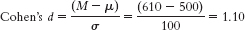
8.9 According to Cohen’s guidelines for interpreting the d statistic, a small effect is around 0.2, a medium effect is around 0.5, and a large effect is around 0.8.
8.11 In everyday language, we use the word power to mean either an ability to get something done or an ability to make others do things. Statisticians use the word power to refer to the ability to detect an effect, given that one exists.
8.13 80%
8.15 A researcher could increase statistical power by (1) increasing the alpha level; (2) performing a one-tailed test instead of a two-tailed test; (3) increasing the sample size; (4) maximizing the difference in the levels of the independent variable (e.g., giving a larger dose of a medication); (5) decreasing variability in the distributions by using, for example, reliable measures and homogeneous samples. Researchers want statistical power in their studies, and each of these techniques increases the probability of discovering an effect that genuinely exists. In many instances, the most practical way to increase statistical power is (3) to increase the sample size.
8.17 The goal of a meta-analysis is to find the mean of the effect sizes from many different studies that all manipulated the same independent variable and measured the same dependent variable.
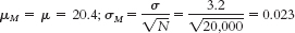
8.19 The file drawer analysis allows us to calculate the number of studies with null results that would have to exist so that a mean effect size would no longer be statistically significant. If it would take many studies (e.g., hundreds) in order to render the effect nonsignificant, then a statistically significant meta-analysis finding would be more persuasive. Specifically, we would be more convinced that a mean effect size really is statistically significantly different from zero.
8.21(i) σ_M is incorrect. (ii) The correct symbol is σ. (iii) Because we are calculating Cohen’s d, a measure of effect size, we divide by the standard deviation, σ, not the standard error of the mean. We use standard deviation rather than standard error because effect size is independent of sample size.
8.23 18.5% to 25.5% of respondents were suspicious of steroid use among swimmers.
8.25
- a. 20%
- b. 15%
- c. 1%
8.27
- a. A z of 0.84 leaves 19.77% in the tail.
- b. A z of 1.04 leaves 14.92% in the tail.
- c. A z of 2.33 leaves 0.99% in the tail.
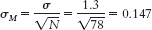
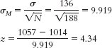
8.29 We know that the cutoffs for the 95% confidence interval are z = ±1.96. The standard error is calculated as:

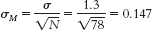
Now we can calculate the lower and upper bounds of the confidence interval.
C-23
M_lower = −z(σ_M) + M_sample = −1.96(0.147) + 4.1 = 3.812 hours
M_upper = −z(σ_M) + M_sample = −1.96(0.147) + 4.1 = 4.388 hours
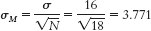
The 95% confidence interval can be expressed as [3.81, 4.39].
8.31z values of ±2.58 put 0.49% in each tail, without going over, so we will use those as the critical values for the 99% confidence interval. The standard error is calculated as:

Now we can calculate the lower and upper bounds of the confidence interval.
M_lower = −z(σ_M) + M_sample = −2.58(0.147) + 4.1 = 3.721 hours
M_upper = −z(σ_M) + M_sample = −2.58(0.147) + 4.1 = 4.479 hours
The 99% confidence interval can be expressed as [3.72, 4.48].
8.33
- a.
- b.
- c.
8.35
- a.
- b.
- c.
8.37
- a. Large
- b. Medium
- c. Small
- d. No effect (very close to zero)
8.39
- a. The percentage beyond the z statistic of 2.23 is 1.29%. Doubled to take into account both tails, this is 2.58%. Converted to a proportion by dividing by 100, we get a p value of 0.0258, or 0.03.
- b. For −1.82, the percentage in the tail is 3.44%. Doubled, it is 6.88%. As a proportion, it is 0.0688, or 0.07.
- c. For 0.33, the percentage in the tail is 37.07%. Doubled, it is 74.14%. As a proportion, it is 0.7414, or 0.74.
8.41 We would fail to reject the null hypothesis because the confidence interval around the mean effect size includes 0.
8.43 Your friend is not considering the fact that the two distributions, that of IQ scores of Burakumin and that of IQ scores of other Japanese, will have a great deal of overlap. The fact that one mean is higher than another does not imply that all members of one group have higher IQ scores than all members of another group. Any individual member of either group, such as your friend’s former student, might fall well above the mean for his or her group (and the other group) or well below the mean for his or her group (and the other group). Research reports that do not give an indication of the overlap between two distributions risk misleading their audience.
8.45
- a. Step 3:
  
  Step 4: The cutoff z statistics are +1.96 and 1.96.
  Step 5: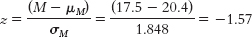
  
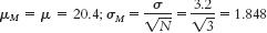
  Step 6: Fail to reject the null hypothesis; we can conclude only that there is not sufficient evidence that Canadian adults have different average GNT scores from English adults. The conclusion has changed, but the actual difference between groups has not. The smaller sample size led to a larger standard error and a smaller test statistic. This makes sense because an extreme mean based on just a few participants is more likely to have occurred by chance than is an extreme mean based on many participants.
- b. Step 3:
  
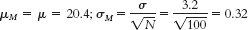
  Step 5: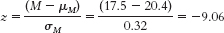
  
  Step 6: Reject the null hypothesis. It appears that Canadian adults have lower average GNT scores than English adults. The test statistic has increased along with the increase in sample size.
- c. Step 3:
  Step 5:
  
  The test statistic is now even larger, as the sample size has grown even larger. Step 6 is the same as in part (b).
- d. As sample size increases, the test statistic increases. A mean difference based on a very small sample could have occurred just by chance. Based on a very large sample, that same mean difference is less likely to have occurred just by chance.
- e. The underlying difference between groups has not changed. This might pose a problem for hypothesis testing because the same mean difference is statistically significant under some circumstances but not others. A very large test statistic might not indicate a very large difference between means; therefore, a statistically significant difference might not be an important difference.
8.47
- a. No, we cannot tell which student will do better on the LSAT. It is likely that the distributions of LSAT scores for the two groups (humanities majors and social science majors) have a great deal of overlap. Just because one group, on average, does better than another group does not mean that every student in one group does better than every student in another group.
  C-24
- b. Answers to this will vary, but the two distributions should overlap and the mean of the distribution for the social sciences majors should be farther to the right (i.e., higher) than the mean of the distribution for the humanities majors.
8.49
- a. Given μ = 16.189 and σ = 12.128,
  we calculate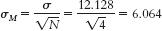 , we calculate = 6.064. To calculate the 95% confidence interval, we find the z values that mark off the most extreme 0.025 in each tail, which are −1.96 and 1.96. We calculate the lower end of the interval as M_lower = −z(σ_M) + M_sample = −1.96(6.064) + 8.75 = −3.14 and the upper end of the interval as M_upper = z(σ_M) + M_sample = 1.96(6.064) + 8.75 = 20.64. The confidence interval around the mean of 8.75 is [−3.14, 20.64].
- b. Because 16.189, the null-hypothesized value of the population mean, falls within this confidence interval, it is plausible that the point spreads of FCS schools are the same, on average, as the point spreads of FBS schools. It is plausible that they come from the same population of point spreads.
- c. Because the confidence interval includes 16.189, we know that we would fail to reject the null hypothesis if we conducted a hypothesis test. It is plausible that the sample came from a population with μ = 16.189. We do not have sufficient evidence to conclude that the point spreads of FCS schools are from a different population than the point spreads of FBS schools.
- d. In addition to letting us know that it is plausible that the FCS point spreads are from the same population as those for the FBS schools, the confidence interval tells us a range of plausible values for the mean point spread.
8.51
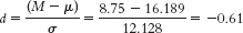
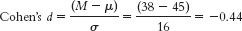
- a. The appropriate measure of effect size for a z statistic is Cohen’s d, which is calculated as
- b. Based on Cohen’s conventions, this is a medium-to-large effect size.
- c. The hypothesis test tells us only whether a sample mean is likely to have been obtained by chance, whereas the effect size gives us the additional information of how much overlap there is between the distributions. Cohen’s d, in particular, tells us how far apart two means are in terms of standard deviation. Because it’s based on standard deviation, not standard error, Cohen’s d is independent of sample size and therefore has the added benefit of allowing us to compare across studies. In summary, effect size tells us the magnitude of the effect, giving us a sense of how important or practical this finding is, and allows us to standardize the results of the study. Here, we know that there’s a medium-to-large effect.
8.53
- a. We know that the cutoffs for the 95% confidence interval are z = ±1.96. Standard error is calculated as:
  
  Now we can calculate the lower and upper bounds of the confidence interval.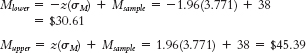
  
  The 95% confidence interval can be expressed as [$30.61, $45.39].
- b. Standard error is now calculated as:
  
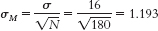
  Now we can calculate the lower and upper bounds of the confidence interval.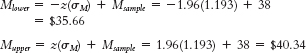
  
  The 95% confidence interval can be expressed as [$35.66, $40.34].
- c. The null-hypothesized mean of $45 falls in the 95% confidence interval when N is 18. Because of this, we cannot claim that things were lower in 2009 than what we would normally expect. When N is increased to 180, the confidence interval becomes narrower because standard error is reduced. As a result, the mean of $45 no longer falls within the interval, and we can now conclude that Valentine’s Day spending was different in 2009 from what was expected based on previous population data.
- d. , just around a medium effect size.
8.55
- a. Standard error is calculated as:
  
  Now we can calculate the lower and upper bounds of the confidence interval.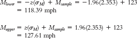
  
  The 95% confidence interval can be expressed as [118.39, 127.61].
  Because the population mean of 118 mph does not fall within the confidence interval around the new mean, we can conclude that the program had an impact. In fact, we can conclude that the program seemed to increase the average speed of women’s serves.
- b. 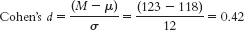, a medium effect.
- c. Because standard error, which utilizes sample size in its calculation, is part of the calculations for confidence interval, the interval becomes narrower as the sample size increases; however, because sample size is eliminated from the calculation of effect size, the effect size does not change.
C-25
8.57
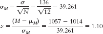
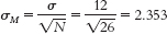
- a. Step 1: We know the following about population 2: μ = 118 mph and σ = 12 mph. We know the following about population 1: N = 26 and M = 123 mph. Standard error is calculated as:
  
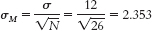
  Step 2: Because we are testing whether the sample hits a tennis ball faster, we will conduct a one-tailed test focused on the high end of the distribution.
  We need to find the cutoff that marks where 5% of the data fall in the tail of population 2. We know that the critical z value for a one-tailed test is +1.64. Using that z, we can calculate a raw score.
  M = z(σ_M) + μ_M = +1.64(2.353) + 118 = 121.859 mph
  This mean of 121.859 mph marks the point beyond which 5% of all means based on samples of 26 observations will fall, assuming that population 2 is true.
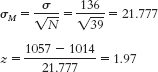
  Step 3: For the second distribution, centered around 123 mph, we need to calculate how often means of 121.859 (the cutoff) and more occur. We do this by calculating the z statistic for the raw mean of 121.859 with respect to the sample mean of 123.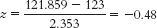
  
  We now look up this z statistic on the table and find that 18.44% falls between this negative z and the mean. We add this to the 50% that falls between the mean and the high tail to get our power of 68.44%.
- b. At an alpha of 10%, the critical value moves to +1.28. This changes the following calculations:
  M = z(σ_M) + μ_M = +1.28(2.353) + 118 = 121.012 mph
  This new mean of 121.012 mph marks the point beyond which 10% of all means based on samples of 26 observations will fall, assuming that population 2 is true.
  For the second distribution, centered around 123 mph, we need to calculate how often means of 121.012 (the cutoff) or larger occur. We do this by calculating the z statistic for the raw mean of 121.012 with respect to the sample mean of 123.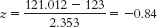
  
  We look up this z statistic on the table and find that 29.95% falls between this negative z and the mean. We add this to the 50% that falls between the mean and the high tail to get power of 79.95%.
- c. Power has moved from 68.44% at alpha of 0.05 to 79.95% at alpha of 0.10. As alpha increased, so did power.
8.59
- a. The topic is the effectiveness of culturally adapted therapies.
- b. The researchers used Cohen’s d as a measure of effect size for each study in the analysis.
- c. The mean effect size they found was 0.45. According to Cohen’s conventions, this is a medium effect.
- d. The researchers could use the group means and standard deviations to calculate a measure of effect size.
8.61
- a. A statistically significant difference just indicates that the difference between the means is unlikely to be due to chance. It does not tell us that there is no overlap in the distributions of the two populations we are considering. It is likely that there is overlap between the distributions and that some players with three children actually perform better than some players with two or fewer children. The drawings of distributions will vary; the two curves will overlap, but the mean of the distribution representing two or fewer children should be farther to the right than the mean of the distribution representing three or more children.
- b. A difference can be statistically significant even if it is very small. In fact, if there are enough observations in a sample, even a tiny difference will approach statistical significance. Statistical significance does not indicate the importance or size of an effect—we need measures of effect size, which are not influenced by sample size, to understand the importance of an effect. These measures of effect size allow us to compare different predictors of performance. For example, in this case, it is likely that other aspects of a player’s stats are more strongly associated with his performance and therefore would have a larger effect size. We could make the decision about whom to include in the fantasy team on the basis of the largest predictors of performance.
- c. Even if the association is true, we cannot conclude that having a third child causes a decline in baseball performance. There are a number of possible causal explanations for this relation. It could be the reverse; perhaps those players who are not performing as well in their careers end up devoting more time to family, so not playing well could lead to having more children. Alternatively, a third variable could explain both (a) having three children, and (b) poorer baseball performance. For example, perhaps less competitive or more laid-back players have more children and also perform more poorly.
- d. The sample size for this analysis is likely small, so the statistical power to detect an effect is likely small as well.
8.63
- a. The sample is the group of low-income students utilized for the study by Hoxby and Turner (2013). The population is low-income students applying to college.
- b. The independent variable is intervention, with two levels—no intervention and intervention.
- c. The dependent variable is number of applications submitted.
- d. Just because a finding is statistically significant, it does not mean that it is practically significant. Justification for the impact of using the intervention based on cost-benefit may be needed.
- e. The effect size for number of applications submitted was 0.247. This is a small effect size according to Cohen’s conventions.
- f. Effect sizes demonstrate the difference between two means in terms of standard deviations. Thus, for the number of applications submitted, the means for the two groups were 0.247 standard deviations apart.
- g. The intervention increased the average number of applications submitted by 19%.

C-26