Chapter 13 How it Works
13.1 Conducting A One-Way Within-Groups ANOVA
Researchers followed the progress of 42 people undergoing inpatient rehabilitation following a spinal cord injury (White, Driver, & Warren, 2010). They assessed the patients on a variety of measures on three separate occasions—
| Admission | Three Weeks | Discharge | |
|---|---|---|---|
| Patient 1 | 6.1 | 5.5 | 5.3 |
| Patient 2 | 6.9 | 5.7 | 4.2 |
| Patient 3 | 7.4 | 6.5 | 4.9 |
How can we use one-
- Population 1: People just admitted to an inpatient rehabilitation facility following a spinal cord injury. Population 2: People 3 weeks after they were admitted to an inpatient rehabilitation facility following a spinal cord injury. Population 3: People being discharged from an inpatient rehabilitation facility following spinal cord injury.
The comparison distribution will be an F distribution. The hypothesis test will be a one-way within- groups ANOVA. Regarding the assumptions: (1) The patients were not selected randomly (all were from the same hospital), so we must generalize with caution. (2) We do not know if the underlying population distributions are normal, but the sample data do not indicate severe skew. (3) To see if we meet the homoscedasticity assumption, we will check to see if the variances are similar (typically, when the largest variance is not more than twice the smallest) when we calculate the test statistic. (4) The experimenter could not counterbalance, so order effects might be present. With different levels of a time- related variable, it is not possible to assign someone to be measured at, for example, the final time point before the first time point. - Null hypothesis: People in an inpatient rehabilitation hospital for a spinal cord injury have the same levels of depression, on average, at admission, 3 weeks later, and at discharge—
H0: μ1 = μ2 = μ3. Research hypothesis: People in an inpatient rehabilitation hospital for a spinal cord injury do not have the same levels of depression, on average, at admission, 3 weeks later, and at discharge— H1 is that at least one μ is different from another μ. - We use an F distribution with 2 and 4 degrees of freedom.
dfbetween = Ngroups − 1 = 3 − 1 = 2
dfsubjects = n − 1 = 3 − 1 = 2
dfwithin = (dfbetween)(dfsubjects) = (2)(2) = 4
dftotal = dfbetween + dfsubjects + dfwithin = 2 + 2 + 4 = 8 (or dftotal = Ntotal − 1 = 9 − 1 = 8) - The critical value for the F statistic for a p level of 0.05 and 2 and 4 degrees of freedom is 6.95.
- SStotal = Σ(X − GM)2 = 8.059.
Time X X − GM (X − GM)2 Admission 6.1 0.267 0.071 Admission 6.9 1.067 1.138 Admission 7.4 1.567 2.455 Three weeks 5.5 −0.333 0.111 Three weeks 5.7 −0.133 0.018 Three weeks 6.5 0.667 0.445 Discharge 5.3 −0.533 0.284 Discharge 4.2 −1.633 2.667 Discharge 4.9 −0.933 0.87 GM = 5.833 Σ(X − GM)2 = 8.059 SSbetween = Σ(M − GM)2 = 6.018
Time X Group Mean (M) M − GM (M − GM)2 Admission 6.1 6.8 0.967 0.935 Admission 6.9 6.8 0.967 0.935 Admission 7.4 6.8 0.967 0.935 Three weeks 5.5 5.9 0.067 0.004 Three weeks 5.7 5.9 0.067 0.004 Three weeks 6.5 5.9 0.067 0.004 Discharge 5.3 4.8 −1.033 1.067 Discharge 4.2 4.8 −1.033 1.067 Discharge 4.9 4.8 −1.033 1.067 GM = 5.833 Σ(M − GM)2 = 6.018 SSsubjects = Σ(Mparticipant − GM)2 = 0.846
Participant Time X Participant Mean (Mparticipant) Mparticipant − GM (Mparticipant − GM)2 1 Admission 6.1 5.633 −0.2 0.040 2 Admission 6.9 5.6 −0.233 0.054 3 Admission 7.4 6.267 0.434 0.188 1 Three weeks 5.5 5.633 −0.2 0.040 2 Three weeks 5.7 5.6 −0.233 0.054 3 Three weeks 6.5 6.267 0.434 0.188 1 Discharge 5.3 5.633 −0.2 0.040 2 Discharge 4.2 5.6 −0.233 0.054 3 Discharge 4.9 6.267 0.434 0.188 GM = 5.833 Σ(Mparticipant − GM)2 = 0.846 SSwithin = SStotal − SSbetween − SSsubjects = 8.059 − 6.018 − 0.846 = 1.195
We now have enough information to fill in the first three columns of the source table—
the source, SS, and df columns— and to divide each sum of squares by the degrees of freedom to get variance, MS. 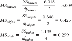
343
We then calculate two F statistics—
one for between- groups and one for subjects— by dividing each MS by the within- groups MS. 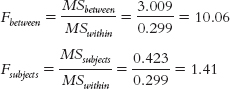
The completed source table is:
Source SS df MS F Between 6.018 2 3.009 10.06 Subjects 0.846 2 0.423 1.41 Within 1.195 4 0.299 Total 8.059 8 We want to know if there’s a statistically significant difference between groups, so we’ll look at the between-
groups F statistic, 10.06. - The F statistic, 10.06, is beyond the critical value, 6.95. We can reject the null hypothesis. It appears that depression scores differ based on the time point during rehabilitation. A post hoc test is necessary to know exactly which pairs of means are significantly different.