Chapter 16 Exercises
Clarifying the Concepts
Question 16.1
hcYdTAmy8tr/vnPQrLlYTozgDiv8scQcViJe/tRxuWzhuMORdCv0J85a5MaSOAe2eFZELZsKHnAGPjmbOKep4JEyH3sQywWY9g1TaQ9UPQCcGFEohUuz2StkA00=Question 16.2
3Xpr+ZlCd+3PBb0dX3ttqRBsMjmJ3MuHWJkQulCBLjtvXc0fa1yYF/1ykhhaQmMZb1Shk1S5jEmSTn4ILXr9J9i1PjshUkDD6qk6YuVUStgyVg3+FC2T1yMDYB4=Question 16.3
9oxDBn3vI+cgYKegLEakT7YvoQw6cZwAoY50l4IOqeaa3IDnd3eSjgrqff/m8XtvN8AF9XeMSUXNrVlMuvUDXrrViwSvyXEjOvVUBRh2Hc87wrEeXPJ03OZ/sARBqEuEMbLmimM7W3FU2LI9uHnfkjIzgIOTb143hgSurSnnOcqNDdg9vhycWdPfwW9/IHChaS4/N7fGbzfu07tqFcBfzxIcsRJvPxW1Z5UmGWpbYFi6J4t6c5Wn/sQ9ZmcSmDANWAvnZcpdNYgA77dqsKSsiUPHFds=Question 16.4
u9u79J83OSBJaJVqoyfgDepZLa1hDR70OCtTme8+sgmHLytcyv9stq5pga7kiov64JbfSPAKbs9PX1K3VxjA7OTRKUQ/iDHXXLQMR4wVFfVxD8GRUf/9liGcSydBXfKqOTVFX0pttNFOJNDLB2aS4PFSbzG9ADjH8k/2Ps8uF83xwJCQ0m4FoEA6HrAWfF4Qb/3qNqLAqabRLZTA3bjmWp++4qHnFAVcJ9jZkTr23/3yIocB4PBIYF0MDq9xFioNwqNimXh4QkSkNOrfab15lLEYfmRY6cD5qYAsn6CibY4OUr/RtA3kuMGYlWk=Question 16.5
6NTX/mReff7huVI00gvkpp45hGPi5FAficaJmwcqbV0iVO9XmEx4gzsCgYLP47yQtXHFkRrDnLGjVACu0liBQ/GKRZsHA3bAAxlTJfUeQ8NJ/mXlD4pNl0DRPm5XxrSrwKrqM/xH8Avcad+SZOrLJMQM0ZGHIFB3dGrCkDBJ2FcVHIDIJuUkhvVN4ZLtYhymrPApjWGJQDfpV6zXTk0EJzey/fgNKi8cgAaJ0R1zLhiOTlBwxXSOuIjuAiGWmSkFBPX9BRth/pbNEU4tllI7AG/DudwJl1YBxkbqUi24Yxr3O5wrkayxZX1lX4t+ZTBvHFpcSjBmO0R+mvDP9KENmQ==Question 16.6
pb/s7W5b+8fOadzuB+oyiZ2S0QltDXg6jJZ7ZaLfsDglpEtgCT5yj1s4c33jR8nFRHKOCzQoDJ3Vm1/7iUEZGvFstNo=Question 16.7
ilNdvBi5D7ZeMF9G6UoSE/QslQNqhuqn0Yk/26DWKC6D6ss5M7mhTjg4LgNnJh0QzPhPxdl7Wrj5JNBMEjs62g==Question 16.8
VK2rdM+taqN4v0kHCBP7kyVNJgNpokDo8J06VP6aMs/DYYRCkCaEP4cJi0U=Question 16.9
cq4N8wZ/kgv7+FhaFoQnbBbkQg0mL/lUAoyWwO+Qp8RbAupf40KU+3g4OqlqFGPSLzD5Y0XxN+EBIt/fhDmrZ05DGkmnIw6k3kWhqTyvXU4=Question 16.10
UTXiaATgZtcLDSzJcVFVD3xnp6Gze0ymV4vp58/mzCf0J6TOEWhI10Ps8YRjdNDEUM1QYKtsHwGYGhe+k2ldcF7S4c3GfItrUDtjob0vaN6ueZ0t1EzTkyCKQb/mXrE2lm+NUw==Question 16.11
e1LPAXCO1CRUKQFoTiVso5cKxhRXv6v35VUz+lwgXw6YQod1ICU8QU4T9LYpBmmP214jjljprE/t7nEHKVupk/08vZ7gqkYA+vkWdX514O//b76tJcEKwjn0mXwQQieqdZfOkR37h84=Question 16.12
aXLMpZHxrfDX+K2WY9sCeymooXMxkL/Ez3xki9sTWQctCINSbNjuGhwA0DNalwnyQY6YQYU+EZ6zMLIT79cZugkMEO/oMihn31ideXzGU3uo5xai/Y/ceOgpF9gMuwC6CTP0inuZ3I/h9RMa4n0wTCOyBE3AfCNulU32nfdrGM8KXPBBK0VbgY1cfFXWRdXhQuestion 16.13
9O/VgkrDnw/jHu1SiN6qD3KmUll4/9u8pN4snH1ILXkN7mmnlT+dApyTqvb6hVwBB4beSPUJEFXqrhxEvNbCadvYtz8IHnYSfCxZwRqWO94myN1VQDJjqHwBYvb+LHs5grh1wIuIq38oGrMZPdlz8OcMO4sfNsxal67rmwHwroiffuxyrMLNzdbjSP3GA7tg/bhfHpE2RQw=Question 16.14
9RYZhM0dMzCjFeJ1Zig7gDG2H1KC7L4vjkXWVSfU5vJil/1aXuBGg6I7m1c3baoxQjIoWfE3pOyqJOThT6yTaWfREEwEk7iExpv3ANOcUAiNMU7wBcZlFLhxtIkC20Vf4k7g2eWWtSo=Question 16.15
4MKiypDw8Tk/7x/tfj5BM5Oi4N1NyeGVB7kKQkiyf4CQ3XjMBiZ/QwfJUjCzumO0+tTaLJ1VUbc=Question 16.16
pY9AmVRQ4eN6NnqS3F+2/UR1FsWft2Ov536Mi/ClVKqANQLC239UlU6PcQTw52n+9lXnU6Lew7fTYgE9AW5B1zlXUStnZpSmRgSrnpDJeXJKvcDSM/rH5BTCmGHLVnrIGoui/WTztozo/GNG2HReTcr3I0tvUqQsdFPuH1TMbjORlothWGUZbfoUwk1aDmEUeJHEfg==Question 16.17
WxRtreDnqEpJdGzgieMY2mjThM7ScojAXJv8RNvZwqxYmhulb9rxFBO8e3kHgCMysXxeDOMA6IdZEWUPxrPd/NeB9fimhpRHQOjAUfdKi0mKp+AW6PrndMRmqys=Question 16.18
dOIq4EQtQb3ETEePSrlCyYpddyHUN1ChYaCM6aVGzQPq6Kg+gFfiVfU6PP/7Yre0iWkhXNWNCjX53SUHs5IKyS9q1AoAwaKcbUAnmJh9UZZDhUA9Question 16.19
Ym6XX2ek6LAsk3koSXE89AJ/+gUPp3VYrf1/G2/QqegKOgaGwCkinVsEx5KJoCohQuestion 16.20
n7SGx1LiM62Jvd1BHo/juBeeV6ZWYHuwVHUMb59EgOkDtWz3VyAba8DYZz6u/qPXEFxkWnKZ8sWp+zANS89tgm1nAuLn/9QbvOeA6GkrsUnTerNh0Xi+HPvvz69RTg8t9PPqwxQKJT2Zm3554AgcX+Nb9rU=Question 16.21
GiwGmEYi16mqQg+Kd88/4r/ikKIciKv2JUVKPye8D9qyLTota0ksXc6glD3il3yr9JmGbObU99yeh296djGD6bdnWCS6LQMmB5v+SDKjP3Ey3pc4L0o8y4SRr+E=452
Question 16.22
i4A4jxpU8zZY762jzW+Zyg9W6SNp7jWkCHtfPZcGHKOQ8LS+iof0SMSgfkxOk8MT9gpQWK421Wu1WKKCgrRwZEbDYxyicFJh4a20VI9JEjWoCqZKlm1KzcVOAck7UK+XQVQpJhire+T05n/t1pfRvdozZbg=Question 16.23
smdyMuVgsU5kKa/kyLPLuxEWOZ4oxUwxos06GITWOb1iNWTsSRrdCyjrxZlUwyzEhkCxH1BHttVFRd+IQbXyo8tDWsBEhzG1Ab7iWjmQV0U=Question 16.24
0UP6OYxpftUtbPkFBC6Bsm1g+t1JQ4Iv7+fFYt1y/AnaszP3aUxPfVKD4pj4xCJD5QRaPXGyJ1PasNF4Ab8C5kBYkTQg2LwIn47DO9hknwAqkuaZXIJHI4jE8z8=Question 16.25
aLUn9L6gzwu1NumzxuOUsu3nRfNdNrupxVxcDsIshul7nHAC+Ybo+MmI3I9JRZy7TyDaQvkPYqApPEZAMaKky2U0+FfaerSMF0FqppbJmD+gBuMbsg55A/6Jcd4=Question 16.26
YpaPda+G/5zUeRoaYm/1DdDM0quMgdgd6CUjeDt/MtY2HUP/CRfvI7vojdAj63Brnqfe2+AivArjs87ugLSh+TJxHpB+TurwqypnGgid7U/qhLpZjCPualURQu7yvlg8cP+TcZpWQhLQwMz2sM2yhDghkLLEBPE9stpsfU94PJieaxfnCalculating the Statistics
Question 16.27
Using the following information, make a prediction for Y, given an X score of 2.9:
Variable X: M = 1.9, SD = 0.6
Variable Y: M = 10, SD = 3.2
Pearson correlation of variables X and Y = 0.31
- Jqy2ozjiov82tpdCPdkbhwH/KXawLO/gNdUiuzLUKp+NMf4vrFkAplrd1prb0Gdx6qCClhWH2MOQRmuSQHm3aIRXsjxZc/SxTxDoBGApvzCrrfm9+8EsOGSwGOs=
- M0KOBXXEaQrYEKQVg9son9D55B4yJRqmAD7Ditsx4nKXQkSjFOEcW8LjZS7zG9YeH9pYzIf5Vr5Afsdh5SGxrL6Xg29acIhCkphlYw==
- 9ATdyCaHbMScGKJZRepmqPJeOKyr5FxJLskPfNhm+H/oi2xHiyg/RFwMBOYGOMr5aNR2fN4FeDeJsARqgZN981gOqJo5X7nSLMF24gnv5NFWhqaQT4C+gyH/Z3xtHvR5
Question 16.28
Using the following information, make a prediction for Y, given an X score of 8:
Variable X: M = 12, SD = 3
Variable Y: M = 74, SD = 18
Pearson correlation of variables X and Y = 0.46
- Jqy2ozjiov82tpdCPdkbhwH/KXawLO/gNdUiuzLUKp+NMf4vrFkAplrd1prb0Gdx6qCClhWH2MOQRmuSQHm3aIRXsjxZc/SxTxDoBGApvzCrrfm9+8EsOGSwGOs=
- Ex+1jXtyPEE4F//zvijdV+R6siSIgGhlVHad0u33UrHfxY5f/EaGI2ioj2y8pnEia9oFyKJHHwHEVjlMI4arigOS1JtqIdbktVU61TgKX0eEfJSz
- 9ATdyCaHbMScGKJZRepmqPJeOKyr5FxJLskPfNhm+H/oi2xHiyg/RFwMBOYGOMr5aNR2fN4FeDeJsARqgZN981gOqJo5X7nSLMF24gnv5NFWhqaQT4C+gyH/Z3xtHvR5
- Wy8612V2bI/F2SqD/cVtlI2bHjIxDggltMNJyQoKCbfQOkvE0x6CSUH8dk62RpdONv22W/SnHtpA11V8wXysWg==
- KS4dtSPxmTyRiyVjmA14/1Pc+MupZ1TDN66jojvXSH0QQNR+hM6RcIJeVLh8a7hP
- L+Bb2pjnvu5RxQwXV3eq5Apb2W7eV/N/8L09bQFoxkAdotgcYX/IKjo5P7pxZgRq
- sDvs6hUCSEd2aMXiKq5G/ubPy5X5WAClPO57fSXfgBZxmbqf21pamOwMmXrmUDOxXVm7253c1qBzmr4QSSnTFuYL5uoXKklrlT8SB5wW/zGAp09/NePSD8AqAZ8bGhGwyozA879FFH9W1wUMWIfpB9AwXH28i/zbtmEW+XV9ZNgTqVzoZi+qfsL4kBc=
Question 16.29
Let’s assume we know that age is related to bone density, with a Pearson correlation coefficient of −0.19. (Notice that the correlation is negative, indicating that bone density tends to be lower at older ages than at younger ages.) Assume we also know the following descriptive statistics:
Age of people studied: 55 years on average, with a standard deviation of 12 years
Bone density of people studied: 1000 mg/cm2 on average, with a standard deviation of 95 mg/cm2
Virginia is 76 years old. What would you predict her bone density to be? To answer this question, complete the following steps:
- Jqy2ozjiov82tpdCPdkbhwH/KXawLO/gNdUiuzLUKp+NMf4vrFkAplrd1prb0Gdx6qCClhWH2MOQRmuSQHm3aIRXsjxZc/SxTxDoBGApvzCrrfm9+8EsOGSwGOs=
- Ex+1jXtyPEE4F//zvijdV+R6siSIgGhlVHad0u33UrHfxY5f/EaGI2ioj2y8pnEia9oFyKJHHwHEVjlMI4arigOS1JtqIdbktVU61TgKX0eEfJSz
- 9ATdyCaHbMScGKJZRepmqPJeOKyr5FxJLskPfNhm+H/oi2xHiyg/RFwMBOYGOMr5aNR2fN4FeDeJsARqgZN981gOqJo5X7nSLMF24gnv5NFWhqaQT4C+gyH/Z3xtHvR5
- Wy8612V2bI/F2SqD/cVtlI2bHjIxDggltMNJyQoKCbfQOkvE0x6CSUH8dk62RpdONv22W/SnHtpA11V8wXysWg==
- KS4dtSPxmTyRiyVjmA14/1Pc+MupZ1TDN66jojvXSH0QQNR+hM6RcIJeVLh8a7hP
- L+Bb2pjnvu5RxQwXV3eq5Apb2W7eV/N/8L09bQFoxkAdotgcYX/IKjo5P7pxZgRq
- sDvs6hUCSEd2aMXiKq5G/ubPy5X5WAClPO57fSXfgBZxmbqf21pamOwMmXrmUDOxXVm7253c1qBzmr4QSSnTFuYL5uoXKklrlT8SB5wW/zGAp09/NePSD8AqAZ8bGhGwyozA879FFH9W1wUMWIfpB9AwXH28i/zbtmEW+XV9ZNgTqVzoZi+qfsL4kBc=
Question 16.30
Given the regression line  = −6 + 0.41(X), make predictions for each of the following:
- 5/FU4SrgisJJmRBE8SWZUqnJvOcpfAiByiZv4QePoVY=
- UDALzQuKKZc/w7lbFjgl/Q8k/rpLnxZczIakqc5XJgE=
- flDrnKVoaWVWKEzsgwV5YKtgf6uDA5fQ2V/O8byKGDc=
Question 16.31
Given the regression line
= 49 − 0.18(X), make predictions for each of the following:
- 9xRYzW7NMhw2UC8A+KR5+HuEOmea5mXlmy+XYL6LP1StsqwV
- YEzmcgf2L9C3SHMYSeJ9ANp2z9HuAbojEkumQ6N78gc=
- wZub5HeNaFNJ3hhHyhnbVmvi7rxySvERUjWyULi3Yzk=
Question 16.32
Data are provided here with descriptive statistics, a correlation coefficient, and a regression equation: r = 0.426,
= 219.974 + 186.595(X).
| X | Y |
|---|---|
| 0.13 | 200.00 |
| 0.27 | 98.00 |
| 0.49 | 543.00 |
| 0.57 | 385.00 |
| 0.84 | 420.00 |
| 1.12 | 312.00 |
| MX = 0.57 | MY = 326.333 |
| SDX = 0.333 | SDY = 145.752 |
Using this information, compute the following estimates of prediction error:
- bcRkmHnRJZ006yRej6xs29Xj0GCiAc9+edlv6PYjCahrE1UywjjY6/t4hot2N3Qaj2JZoGMaIvhokutWrrxTwhquuzeG0bxMcPSrWbpgmcrdwoEWahVUbciVW8sV1+Fv
- rAzABakFGxVgT8aGrj1s1tdb5ZEN8pzovUO3q1so+Tc2XU+9D3BhPJQlQJpxL2qLy7iuuDufneWE8EkPfbBRN/h2teIYsFZQy+W6QSacxAf74vUVXKjwCUzjfHZAxWXsNCWkYPBsK98iAu1ZTVxIdIayZ9vShen5+FnZfbFDnd+RHPOaH/JXKT+6dJUse6Dvl1hJR//G/0oLg0Em
- 2681DKEG0Q7dycq44iZW2ye1SuSX9N+Y38Obsig+exFOSrD9pe1ElYLXY8sQy3Be5SV3FXJDdVpGuXx/5x6Wxv0oLDNAiJCaSliM7CGHGJoRDITb3luqslOuuqs8U0Ia
- CUIXZ6ntEYrGUSnHL7e3ZZV7lpUnsJw2iuNWtEMkMigNPmkh73KeCTM6W/ETuHUPZFdVA0lGnx+JNxz2gJqbeIPWRKKOyxGHV19qe/KJQOELAxigMut440el4kDhWRGL+f0BWty8IMJqYN9Y10H1SjmYl7IwssZu
- pILEic9OghI/SeyhkfD1UaIqmQ+iN3PxW2nL9yU7aEZfgONEQRGz0ZsvPeIhlXofanEihKCDFX0Ap8mV+IrxIA==
Question 16.33
Data are provided here with descriptive statistics, a correlation coefficient, and a regression equation: r = 0.52,
= 2.643 + 0.469(X).
| X | Y |
|---|---|
| 4.00 | 6.00 |
| 6.00 | 3.00 |
| 7.00 | 7.00 |
| 8.00 | 5.00 |
| 9.00 | 4.00 |
| 10.00 | 12.00 |
| 12.00 | 9.00 |
| 14.00 | 8.00 |
| MX = 8.75 | MY = 6.75 |
| SDX = 3.031 | SDY = 2.727 |
Using this information, compute the following estimates of prediction error:
- bcRkmHnRJZ006yRej6xs29Xj0GCiAc9+edlv6PYjCahrE1UywjjY6/t4hot2N3Qaj2JZoGMaIvhokutWrrxTwhquuzeG0bxMcPSrWbpgmcrdwoEWahVUbciVW8sV1+Fv
- rAzABakFGxVgT8aGrj1s1tdb5ZEN8pzovUO3q1so+Tc2XU+9D3BhPJQlQJpxL2qLy7iuuDufneWE8EkPfbBRN/h2teIYsFZQy+W6QSacxAf74vUVXKjwCUzjfHZAxWXsNCWkYPBsK98iAu1ZTVxIdIayZ9vShen5+FnZfbFDnd+RHPOaH/JXKT+6dJUse6Dvl1hJR//G/0oLg0Em
- 2681DKEG0Q7dycq44iZW2ye1SuSX9N+Y38Obsig+exFOSrD9pe1ElYLXY8sQy3Be5SV3FXJDdVpGuXx/5x6Wxv0oLDNAiJCaSliM7CGHGJoRDITb3luqslOuuqs8U0Ia
- CUIXZ6ntEYrGUSnHL7e3ZZV7lpUnsJw2iuNWtEMkMigNPmkh73KeCTM6W/ETuHUPZFdVA0lGnx+JNxz2gJqbeIPWRKKOyxGHV19qe/KJQOELAxigMut440el4kDhWRGL+f0BWty8IMJqYN9Y10H1SjmYl7IwssZu
- pILEic9OghI/SeyhkfD1UaIqmQ+iN3PxW2nL9yU7aEZfgONEQRGz0ZsvPeIhlXofanEihKCDFX0Ap8mV+IrxIA==
Question 16.34
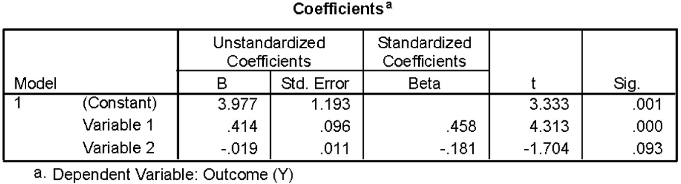
Use this output from a multiple regression analysis to answer the following questions:
- hNfFRgrYZ9m0dbdcGGIBa7k0iXDJjPymKP0+2W4AY7wY+i4MNgL3w2pMR/qIDcnHCpB7zMyR0oawzvg3cb9MSQ==
- tqso8uksy0wqZWGLrzwg6FHTAcDqE8aaUbPO2ex1vPLZgh9Fqysle12YwAkU/+xLVnF+XmJqzEVIPPeYfg0N6P0g9pD7sWN0Ap4N1XwMQVT7R/a40MPX+ybIOao03JBU9AYsvuzowZI=
- Q0u+hU6EK361FFblbFOC7cWHNysI1ZV46GELjGOp/hpE/QBtPXNFVLi3igOA2WLz4oAt8qEfUGyYXCyO7p8F6qLBh1fLZrHxHUukOiEwo3FsotMlBClFlg5HmswkbmAQB9bupFLfipc=
- zq8NkJVbEA4FtqhOUry3hphvRvI2LMgqLH+8H4QgFo1TxsNeEa+PnAHTCrG7ettzsVEjNYKsc7GxuZmRoeank3r8D2QnZVP5JxYgIfRHSjrj48twKfNxnKzqma7vLd+mECJTN9OkhLdk/4uE
Question 16.35
Use this output from a multiple regression analysis to answer the following questions:
- hNfFRgrYZ9m0dbdcGGIBa7k0iXDJjPymKP0+2W4AY7wY+i4MNgL3w2pMR/qIDcnHCpB7zMyR0oawzvg3cb9MSQ==
- o10AjYIdZ8r1v5Evkkvp7gG/DQwduPOB+wApHmuE9k3gctWRtNDmo4ZHycT+QvT/RFl9NIX+WWyKSIwrZYzdqbl6miUChAgBZ29vMnNLVIdQL3wxpTKdMHYwuRY=
- poR8f0RuxqCusg0CHj4/J1CGEya/TbN/c905Iu7oZ/gMapVsSLIVroIfG4/K6W1FG8BGoQbiQ9gyRe2iMRz/WAMrSB7r0Vkv83brdivn5aErgj3DH4oLam9Nps4=
- YKdOZDNGJPxf2mXACKyAmxBnKq/lh5U9eGxBFbeO0YTIKJd8iuu0q2uKQfMm3YPP0iYiGaNfGdl4ZUYBemFaU+gqRWPIBedQAjuSd7qbek8eTg6qNjT/BKkCKsw=
Question 16.36
YIuVtSEhQVBq+z85QOk8KC/kOpv+QDRNkTG2yVPgOxmntByH8J9G25ClTDdgC1iutH5DWxE21f5ITI8wg43q2owaY2gRRmDdXDnDFh7boqHxZTR9hAiQaFaEeuL8ajXG8MZztA4y1WkQ/c+DkWtxrqumjn4KOV+AqRyaMqX3TjVwRwwoXbmQPwwYuS2fSinrSJs/klTUVuvmQEvE5vOswxhX7xdk8upChG5QkDYp1S2ZkK90CodJpiGE4l4U1S1JA0vtHEt41kHlndwjzvylLgphbGoNQRLAIf7+/fbEX89XeV+6L0BJvWv6NnrmbdLlApz4ewfRJory61YovCT1hHiwoGKVkqboWVsoHHgSCbxjDX25pUMlW+8amCQZHm5sK05KT7//UUJLuKO9bVnykR3dmERCB/K53bdUyL6XPA8sYc9i3mEdiddSWgRKccAKnJxD5zsA9yXZqpggt3k7tkIXKk8KtPy4O3i10yIo1yf/8RULFll6SrehQoFq1Eg3d5Sd9MR9GwZLy98lD5+LEMY5URg6kDW9DGzyShHhh2KO2BQGi6qAa0yHYN20Waz5wlg7agiYkaZ6cK17QsRLHjKziWdnGkaJDyuL5y0007euot6Bsfn0XV8aXbPV3o7raZ9oMJViFl5QZIyAGYCGnIC8mA9F0p54Cq441m5zMlVDOhaqRjxhZZ6hkfSmD7K7v6XJTaprAFcf+J0TTHn9aw==Question 16.37
Refer to the structural equation model (SEM) depicted in Figure 16-8 to answer the following:
- N2EeXovV95Hv8qpj9bYv4JPivyT7Nif2JJZujZ+SSXspv6BlvwdQdXCVQRxj2Svx9V6a5tXQY8+0PasuuTKUvkob4udaJTqc27VRYg==
- lsvgg5fUC7Q1M9Z9yz8e1NFY6zMy0iyn+6jmoldc8uEx/EkGpashTSPDR0Tpq/FjODjldwNo717Dw7SYwTjBL9oYIU0xs/a4lwqPXR9tZ1WPrFzZ0XWVVro9UYHusiivWaUlz9fKGMLvRQ0D092L8PQjm0E=
- BaagEK+9ZMbxZ2HGd47keD7rPJ0S/cO/mpzVx5TV09LFLX7MspxjnQORoHsWMSftKRjBosBb/ldE9ERe6tJnU2EXkbqX4qailzpSpsYjpiJWbbj6Nz5UzP1zZebBifc0Mp62kq9KywUCQzJLsm7K52WOnLM=
- xn8Gh1EgkVCuqP/Bzo1rCXjzuMDB5Crs7l3WYMjh2iSZeXYdfuvw+6pDas0q47fIJq2N+el6VVgCI6nG7VKKbsGAgZD77Ui3nLWSieUCwM+ztu+egneXtZmXHkqLe18ni3I6OS2pY/sIraCnv82mWXdSt3Q=
Applying the Concepts
Question 16.38
Weight, blood pressure, and regression: Several studies have found a correlation between weight and blood pressure.
454
- SIuTGtwW+mCHj7Id5WfcUxFXtCIczlJOqmgB6osVCTJefUqXL5fsSMqA8JnYNUVnGZJqKkEiobl2PB0hIfxer275GwwSZvfTJUx4COyx2JEkOM45
- Rz61kqMtCOKO/8tpq026qtZvN7/CILMwrDzKPTa3XBiuStkYqgN0edMhpRnmUK8gChPXjTUPaXnCnGg/7k9th9x/xxsj07ZZHD0Az+32CV4YpBKcOT6JIVDLBqlsBkJHqIi7WzV3lsmdjBZWM46U6AOQAanh41PxjWmVYIuBXiZyhMzisq9ETkXweudr34WFaWE7XHTozZQQqEC/ZrI1eBt2ekLRe4p9dTryxtRhPQsdrBvWoTynhZxqWR090G957scDoE5c8r/0pgc9idaPLvtdwxcV4YjrUR4n82GMSQWmjJJV4kGVN3Cnd7D3sAaQ4rbIoXf3nSI=
- nJPK3FwtPiX2vOw5LZCXdyppuRaCDDStb4vEDcvlZIS0pgnwgA/b1VnamuoauJ+V/DSHFJpBpSoRlA3r6cldjTtXRPIuhtaEYCydmBgeGI4ErIKc5ojcIyuG0mrR1jED
- qKJx2/bX2UEivOBARlZI+3cVZ01Mnm5FzlnloGwFMLJDdOGUajBQ7v39jEXAO2FYnqT4zXLsx6lkIiwS/Dx7NqCfus1T6qYQVISz2WE5P/hI42/nkgYPorJXybNREU+sT9DNEiCMnXUIJ3UEESvir3io89e5XHL86cpaGqleEwd4QbwE0O+rximWBqJgto+PHRTfKolXYas=
Question 16.39
Temperature, hot chocolate sales, and prediction: Running a football stadium involves innumerable predictions. For example, when stocking up on food and beverages for sale at the game, it helps to have an idea of how much will be sold. In the football stadiums in colder climates, stadium managers use expected outdoor temperature to predict sales of hot chocolate.
- RuLM1GiIyQlSGJYeizaYCZ/t4O9kCXlzL1j8w9kbA8JQssTrBorO67rpPZJfmUyF8Yt42VwpoRr+sASdKopmuVqnED8=
- TupEhpJe9+n112TpLjrMVzCs5i7zYEgZh2Q3kuxeEw6wxopC9PUyl5tOzrs3scbN
- UNKmdQl7QRuP1kjtxDpX8FXuElDgZeT64Vf+7fCCnrY0cq0rG3IzfAXOAMQci3W8m+SwecBpc6J5/nE5w5A5TocnUaR+arOQLQYusvjC+nkR0/1M6RYs/MI4pauPXclgyflwvkM09J3Qkrm2lUIMDEAUddMjtLUxLjyVyhRS0FMGwXr3XqzzkS6AOqQ=
- WVwh9/qFHSaukaJLPWsvNYnWx/Vl8miSgbGzOpSVSqwJhEvQZoLHC7u1hPn+vNy93ZcdJP9FcyflbRljmpeqvG0Pc2cvWEPYxUhtUuNKI9p16bh3gMYl3NWFZ990GKfB
Question 16.40
Age, hours studied, and prediction: In How It Works 15.2, we calculated the correlation coefficient between students’ age and number of hours they study per week. The correlation between these two variables is 0.49.
- ffOlrVGUbnrEzwenPR/NWyvpKv4pYYVmW4v1wWPfi7H32fRxWZNAA8L2tbvQ4bey6Bpg+PTdFjDWLR3wsorRJ3brHHIWXfDXBzOxNfal5cadXgG3KRLjPo5rGYQK+nXmxHfDB1ERV8wiC8cgTRZvamYj07V/m+TM1rm3kK2FyzrFEzXBxKrgAvenjj+U4L9uZ3F56AoDYUmj9cRV
- 9NrlX4zkYLI4fsiMSrgMZ+CuY1PdGldBaMqcdZFtGhJF8MivqHUOF1IlDQHwTTZ1fjOdUKu75WP59q0KyJs4HOyQH22MneHV3HgtFRZpyuCOWFSiHrRghW9QA662r3/2lDisVpJCFYIxQELgEyhmh7I8Jz0qLdFTCTnIVaoa4hWRWWsU68qItxK/jabnmKvHelK8Vs7192Y=
- qS2WCinhgFQYsGGJKLJLMaR+e0yTiVKqsInBUsgI292lFe/GpMo784gHACB1JbWMIXA6PQHzQlfzvdw18rGbiAmfj/7SGZ9WnVvhj5Il1+8pYCgVQ+Tn+xGOgl3Ys1LG8GkF1PuXdRRlUG0zlig3E3sT5kBPF9/9CLGmhbFqaum0UCppTKLe4NXlOM5njI3dMSuyiSkWBBo=
- Jcv2vR5BhncEHXVLMo0SgttQoTZPOJp/GPrmL8lbqawABkKhzCCYNheLACWPMMQsFRXb/pWykN739An+A5SjylzagQyXTyG5mWiJ7vtUhVEFxbY3aoe8BdlLvZ4XuD10T3bkID0i1RQb7rhwJUFaTr4NOdzv1qKK/NdkwdDZcRXDg7K4jQCL3FqI2EVVqVn8UAaSqOn9sBw=
Question 16.41
Consideration of Future Consequences scale, z scores, and raw scores: A study of Consideration of Future Consequences (CFC) found a mean score of 3.51, with a standard deviation of 0.61, for the 664 students in the sample (Petrocelli, 2003).
- P+mkLLhZzBCPNGE0cgWU6IRnuYOLT6sdJ0vXU0So/p/e5aoZMu3DCqH+GfV0SKg8DZUpq70liPk4aUZKSXMivqGNK3X59kErZE2dxzOjSHOA5zzwQCwI07ReAMhLdstWKQBiO1Z236U3VO51MTRU5IdNBmwZ4wVGG9tgwXmaoJE/oVxr9Ue4vt85AilJghFINOU5k2DO8qjLhiZwYBkB1UlUcCIdot4u4gaAHC5KlsBSrmPajpKVhqSa8mo=
- X4xEgnLgoI4Mo6b40gBpr/JhnVxdw8alDMC30c1ikSmRKinecWcT25c9QtJDfD4XkcNIvizkBrJpTR0xaSW7lR6QrkY+Z8THmLPkGzaHqu8oWZLNArecjG4G/5BxJl5kz4yFskxR2kiyiW0qtXgbpfJyCWM6kTBnF0fIGD67g+gngmdYAGxkPGYlE1s4/5iDK5ELvrN9doBdfxwo9dq1ZenaKiBsKP7jieUEfBrT1BFqgLtEek6Opg==
Question 16.42
The GRE, z scores, and raw scores: The verbal subtest of the Graduate Record Examination (GRE) has a population mean of 500 and a population standard deviation of 100 by design (the quantitative subtest has the same mean and standard deviation).
- yCBqWsrlSlgeNWpjoDAvqW1gVfobVi0hC2djWxFOMHeMswvI8jEz5NjumYwSEjZmFEHNFlaHZdtoIdeeW1vEC1BUjFKnM/pewFrgXBH9+JkQ7pSsqzrPyx8MVk5Z8TUxVmKH11CdzQ9ksXzBqhQcGdyGdwlpKDxg+ObjgVm615AOA4ddPFGlQSyuRqc=
- oA3u/JaKmHHy2soDSSoH0HcHd7k7F7ssQZM5P8iE8skerludaMYDV75UnTP1j6/ruj9jltetkWKyJ+IpcfmPZy8OTHGftqp+AVNGrdunb46wM+QyyC43ECni6NxtdIUT04xjFT7yRmFuW5cSk4vWMiF0JYgz/lesJpdmI5FYSbW+Rv+lBzrmqQclMST7W+Ra
Question 16.43
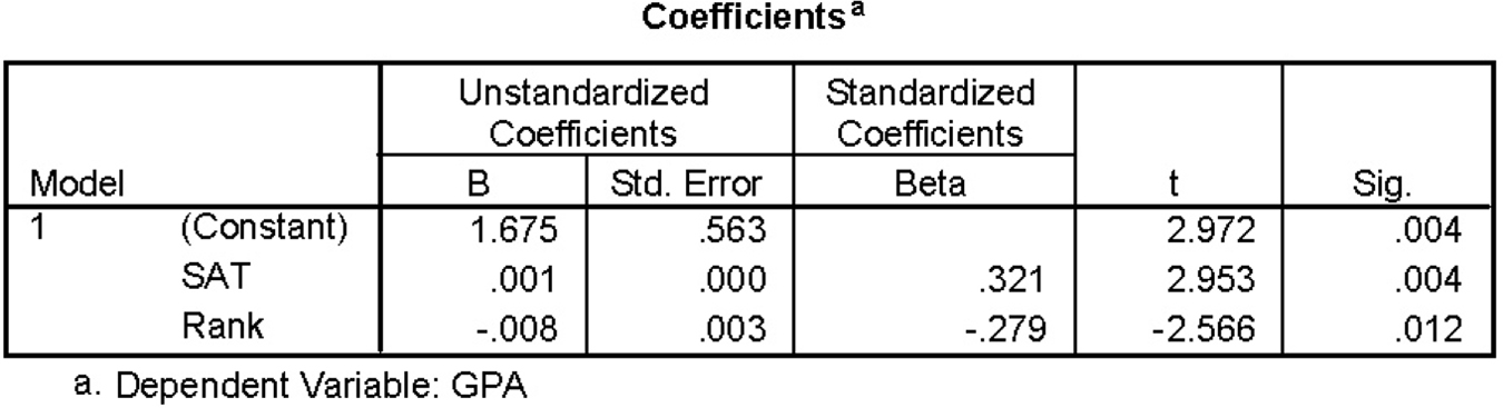
Hours studied, grade, and regression: A regression analysis of data from some of our statistics classes yielded the following regression equation for the independent variable (hours studied) and the dependent variable (grade point average [GPA]):
= 2.96 + 0.02(X).
- MLsATpX8Vu7NN1SrgdFzS3hq+1rc6OpRkgQpgZ+2b3Q+fCv2JnJzWEGbO3bGeV2HzeelkjNVrR0K1fOkGp+rmnLLzli87tIVpoInUWCBWypJIthHTy1iyOgyPS070l9u
- Or6xBMAiUtIhXN3KkDd1UnkSX09W6RxUBw6tiUkj/isslZsUwNphCZ+MPJSpOPAHSiuLoBW5tAvT2w8JvXLnjTJYtjpHkuUq9ejBnT4ZDftjjQIf51BVkx/mnnrjpRx1
- 6lKGnUN8Dd2FMs+7e/oheN4Mnlujl57On3i+52R7vLhZH2mI1BQytQZXT9r4cVEEJxtnY5USP7JziZlswByMAhzkuvRvF1rMSidBXpjZtb9dqInpMm0Gz0Wvk8myfGq5
- CU9jG04iTnU0c0uAFTFy+yYDssijF3ORrFMdPr/bv9QFFEb4nrzr60xLakbArMl9XOvRwJWFDHqSg+HhTD+KQzay9KjEWUq3yfWvQnzxSCq2TXg3g6/IEkA1Fj3JOtM1faPPkQ==
- 5B7QqNsXGnCwWe/LWsAKtX+wTUt3YJFkRF3m1vVBskk8+zoJehxXVMesOxUd6YkfIx9shFNzUrpNWR8dmbsjYFRbzLuWm2rpmL/sLCxR9DoJd4PBTCOL4SIw/pKUCpL7F4Wg8DzuXTuF4dYkIzFQcDg/M7TNYM3kT87yl2wFJYFnzLxLpmUBBALmHA5iT5MMG/Hijaj420Pau6zfhq98hgzMy7OF5k0N4Gk9RWWuAl+melc8gzsgQczY113v5T3++3m9I+OPEMC6Ypx16fvBViExFlMZx/44hxGFCk5ZgAmM5fGKJbAndsl2qDcbBc7l
Question 16.44
Precipitation, violence, and limitations of regression: Does the level of precipitation predict violence? Dubner and Levitt (2006b) reported on various studies that found links between rain and violence. They mentioned one study by Miguel, Satyanath, and Sergenti that found that decreased rain was linked with an increased likelihood of civil war across a number of African countries they examined. Referring to the study’s authors, Dubner and Levitt state, “The causal effect of a drought, they argue, was frighteningly strong.”
- JNyPWFiHQwOQH2A/TiI1K922W/4Vcc2e1KP0FPRQRztxN39lnEK2d1/I2M2C83aQSZof5S2PS0WYQQNQ8gtOfw==
- TupEhpJe9+n112TpLjrMVzCs5i7zYEgZh2Q3kuxeEw6wxopC9PUyl5tOzrs3scbN
- NzQ9cTDkqtuRu7GOHytvbdNZedZBVKnzvy4GwCEO1C7Dw6ZfB/dzvvWEcZ+0i/VD2RkymkIzkYHlN8GdF9DB2kRYWKw+k3lkWJnVCm+Yp0lDYVyBP8mTiWvVAhrnwme4Fd/b/BPIbQ/oGDekQnxk0j1Emp34VuWsksKNSVbAa+vS+R1sni8PcjaxecFUa+ZP2dAF+RW5dQ7GKGhH9h6y7ajsg6vAOybefXHRnAYjCVgzpXzHLvM7vmJ0wwvCxqXD293EZGxKV7Z8w1/JY1Y0xXso6Re2+QzHoLpEq+4zhZn75lAV5ZezaJwhp41eeQrGQtGNwfOiXrWVJer4
Question 16.45
Cola consumption, bone mineral density, and limitations of regression: Does one’s cola consumption predict one’s bone mineral density? Using regression analyses, nutrition researchers found that older women who drank more cola (but not more of other carbonated drinks) tended to have lower bone mineral density, a risk factor for osteoporosis (Tucker, Morita, Qiao, Hannan, Cupples, & Kiel, 2006). Cola intake, therefore, does seem to predict bone mineral density.
455
- Ozw6MHWvkJKjaO6O7HOn1l8iBM9PDSOtDnQSW7bIi5U8BDWGKIqOUC2wXLKk2cTtK11sE5b4zcCz0uLKJzNKV0PMifU8KHRJ8hNCenwN+yVoT/+fnq5sRMs0otkpUX0rbKaJ66og85OsVlyz
- 4NumJ6tv64yDyKprOuS7/+RwJeDFyYiAs1BeGJWYAIth068tmfEvEpGtXTZAaxt3U93KxheEBfhdQPy8XiC3BJI700D9RXRAeEqaP1OJ9Xtx1/l1o1NDXEAjRoEGCwaS7gGz+GXqdovxwisXm7WmpoGf3JwmhvzqKgP+ET9oxkCi/yjH3F2s8dwC+Ctty/6mx8Yx548fCwgVYoCr4mEeMec1IY5lbyOwUNZrVCFORFTrwKDba7pK1U/R9edBO8DO/2EZrbF8UfsONSzn9O9l0n6lK49jJZd6fBmqAzFZ/OkYLcxc9gfKZxHsJS6Nylm5pJKcYJmk+AJPZsrZEdWuJWJ8uB5RL/fKuurz3gLUlqYYTX87XpkX/nA1ifW5IowCxlLiztJFeTYOZmnIL28uhlwudcb86uLiajl8W31x2VZ76n+Jiaelj3SsoH4etrQ7TZdOcRSqF93z4z1MeDat4Pg7CPuq4goZFDSPy3ZJSzc=
- 5aUS2EgbanRFiEt/ne9EdkGTrOMw6QkZFjyhen78B1+3CcWto7WgGq8+6wGgsUJbDqKPAaHcnQQcYQBQzEMuE1MMV4bAgKXFORKxnYXUnPucsEWPLm1gpCTRYPtRqyqEWT3uhm1sjix3WaR7UDbf+9kqkg3txZRRYQpn/MTA43PoElOl7mSsbvy0OiOvDtlwQiOI8saxSQE=
- 3vjmVDptzQ7VuO2Rth0XCwDG4S7NJYVRKo+ost3+EJTCPMl8KhmCLMAHyyay4kHOQMs5xA6m1GL02G34MOJeQXcK1u+9IPHj/QBLffP47fk0jLS3I8OJ1G06mIMUc7vZYQpdjhWJEo+wZOHEdFwbVMi5cluE+sF1po5nzGQHGkqaT4K9OCFgda9kTZWE2RaoQMENPw==
Question 16.46
Tutoring, mathematics performance, and problems with regression: A researcher conducted a study in which children with problems lear ning mathematics were offered the opportunity to purchase time with special tutors. The number of weeks that children met with their tutors varied from 1 to 20. He found that the number of weeks of tutoring predicted these children’s mathematics performance and recommended that parents of such children send them for tutoring.
- lBFixU0py98+lTzR4ehXR13DBDdjrREatZsvFUJdBBHBvQApiyKVyyqSaNWF56mrau9oqgUOijvcjBUhtqnoXls2I7DdujQowLKQY70dQyk=
- EOLSyX6L5Ev7h2pooJnhvjj9NFwyOvyCvnFDVonu/trcYFiIxTl4S8W9eB7IycsKYfiuAy+BeSBgF25kd6ZfOLuECksI4OdgUOBntEYW1cO+h+ywMPfXd2V83glC2scjvUnbQ+29dQmLTcSmnMBUiOfQdd2qI84BWdNSyWjt56xHHPMr0OfTRaMJbBjwAcDSCxRZLpHosKAVE4uRdbduJo1LwMqDBdYKz1PRQ1A0ba3RO6LUkiWHG8TK2FUUxps9R7Z2tI4txQnIi2xEVnwo+kWtBfWUsFjAn0Ew6wO218uAhO+rtF3tGiDqGcfq2k2SIbzYUxmMlSnXwLRL2rPiCyLxmnnU++R7A4of6l5XTzakac42ckGQHdUyVNNX/opOjjY3ZCo3pabH0fTTzB4/NwSnYRBZXHt4skCe39tx+LeHYsubILdDqRWuZhjNCVSS7ZsXGqy6pbLRfvcRdn98qYkCqJEVg4CaQmSOWtvv0JU=
- GOiE8NNASsilPMH0VRW8lpXK/6GDH8gq1SOUAlchfG0yClcndzCLEX5lxjUoEkdvC6xIfq28t+grGVspEZ0nqQwa03n/FIFc6qvehONyAkMk9FiWFrOBlxlpFkTlx5G8/2r2BbuD/BizKcL96Od4TZMU7K1sEOyplC969scV8y9PJtatXIyvIQj1NIYc63ZcIKOQ+CaxhFSuPyItpX3nbdROmfYBs+G3ZKOzFS+aAsp8fTOPEUMQma49JsgCBOY/tdVHHnj0h1o6V+SHUocmCWw8nd2LggQWejy/3NxtNGvL6zUr+h+HQgzmo9j/9HSBGs+0F7iQbYhwn4gsI252s1D3TPHX0nVK
- bnAmhM7gReu029LpvLnI9pXSF99jDpgfuq61BKdCsqB5TnGqFU+O52cn539zB5dmrGEAkub2gMwNLV/GPbEooAxs7yCn3sS81Ix/+p7kRsn5r9y/UsGGhPzwr9b5vk6o6eb7HCU7Ty1fSHrweU/vGqP/uXbXi0UnFh19yvXCXv9wJwGjRIdHqJa+7cdXXN28MyWWIHOJnsHOCGEEtJxOISyC6dAQ5ISWYbmgxdzxEW/bj1LjyqqZGwqyaRuwaavBgLVbqZYP19+XvhRe9I3Xx/8sAe/Nw+Spe8PIIJLIh8eq4MIGjM5wQlt2NuqMk+uWsmYBqLZfAYezwtg7zvcrXi+dFZMu4VYR98jyCFFvd+0=
- /vbGfuY3httRVYSDh23FzjGGP7emG88S4iikkt5XYrrdDYxqKuCvwzbyh70yY6FCtg8kUIZ80ujsqLBfU1er1eiJx8HC+QiPhchsTYKZxJ35XZuyEoP+I78klASlPWJS
- jo3or0m4EQpViBHg8o1Q6IBs30BMDzVwVIYKgbYoTQIoUQSO0KkxXkMMexBP74Nlu8/oJNHDzshTNndQ8TaaGfCoW+aK08hOtqeX7UgzB5Gv1K43POzNo2GUHnmIEiMrarmiLg==
Question 16.47
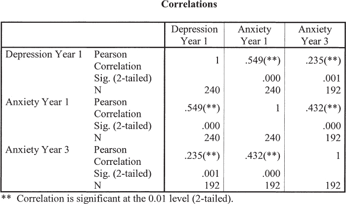
Anxiety, depression, and simple linear regression: We analyzed data from a larger data set that one of the authors used for previous research (Nolan, Flynn, & Garber, 2003). In the current analyses, we used regression to look at factors that predict anxiety over a 3-
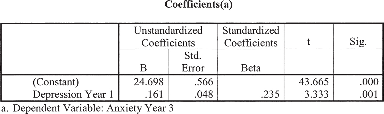
- TybsUH3AwXSqJU991R8g9HQ7vvM9iI5ld+Lwm77IGoIa2ws3TLdkMqAath4TwKZsxXgGXxWpm14mZoE0Fc2r7CfkTHVR7QL1o15Cmw==
- pkyqR5UIBv6Sb5fd/bEtJDbEsWBEZ089pfpRx5i+pJ7REHk3UxwMs6iUd/9OvdJ4g0ekhkGVxnNCnGfaV+x8Fyf6c3RUuS1M3QGbAVRArnWNgMlUCBjB8Ck98Ftgv1DX7v4swpsa0jGkvKTJ/QStyxpWHYBRZmU1MdfUYsmbR4r0k9Cc
- 9Hdr9ZJ/MqCe0NCW3L8Jiqw+RgarT45iVSApP9Wi+/SXGFNkN3Ym8psvO2hsnc6Aefl/okmhoMGUxfu2NoubYV6gwNiOqBZiEzxl8MRk+BZGmr9ipD4C4QOTj8LkZSjPBh8ueUgoisJ3eURd+NDKiuKDCCTJGDZBUMSWfg==
- 7IM3iMvHC7djqlbegVGgHmvQj3mNrZ3ODNY06cXdoYkmqUS6BIhHHx8QMZ5QwF24zom1IjqZihY3clX2HVW3BGeiza84t76Uhu0e41UIrvCHgekT/J40RhkJiJnkLHTQQNhcwhxUVY+37p5DejQbxMWQsPXDSfP/
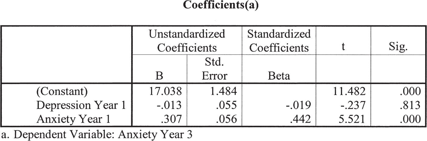
Question 16.48
Anxiety, depression, and multiple regression: We conducted a second regression analysis on the data from Exercise 16.47. In addition to depression at year 1, we included a second independent variable to predict anxiety at year 3. We also included anxiety at year 1. (We might expect that the best predictor of anxiety at a later point in time is one’s anxiety at an earlier point in time.) Here is the output for that analysis.
456
- TybsUH3AwXSqJU991R8g9HQ7vvM9iI5ld+Lwm77IGoIa2ws3TLdkMqAath4TwKZsxXgGXxWpm14mZoE0Fc2r7CfkTHVR7QL1o15Cmw==
- spv1mRHoRK4XXbb9MXxLR9Qfwah5fkJc0xzlbLzAv3/GFv2LCxaUsjYqDXDoO27klJBAW2bTnLLjdKaN2YoOmVwGyD5L8nFVzsSYjBSuH9XG04L2gZECAUvZg70Vs9moZslHQ4mE5LZWZZADIWnA4UD7bu4KMoNNZKq+YxLq542838e9cW5TcMi4AbVTqrTAcGIkHB+8bi0=
- Tz4VS6JVFehymCm0oK1XjjvHKl3PdbSYgvZ4JhF07iEHv0Zjn00Dy5ad+MTNlOHPiUFTmAJRDx4nwDFah4WNYYQrGLB5Mcp7cSJsbq0U/F+4bF48oERiVnsNpTqM5LGUNpZgk8PrcEO9w3oK1O++/x1wq5kN5Tfs8w9n7+HBTyoxx2oveUwKdJCm9i6eAGJsFI4/0atiPYM=
- tOcxqxwDMJ2kawQwR79K31Dh1OEZKfxkjkIBd7eNK3UY3S45MbWUG12XguU65dqxhnm+JvsA8AnzqVzPs6UF6UAFqiLBJlgNm5OR2Nxja3ZsjEEPbT7neAogb2dCTho2u+yS8lCaeEvH+Su5mQ5LJuIVjUUVZTUU0e0vnYufdGTGEYZkDT/gSXuglvjUP25KeyZscky7asa/ke7XDYZmm0lJj5qduaDHI2ynqpOVbkefV1Gu3v4VnkNdU4OXU3k6ZsP8WRsKNBPb1wq2dGEgmcxiiFHvklYvJedyT3JPdH7a5ezgfgmikFIJfkfPuQ9KKVE0bhGKTemkPa1t+zLMEDHTEm2mRU5zJWeBTHckBY76DKodMvosUqGZY6zcORYW/LJ+4U/nhsCKfIX7i/MqgGJWZ354x+p5/dW/P0wuWj3VYN3LyMQZS6ShmwFRhy5NDrbvKJqw9j0vE8mZs7ER/Lh+goFzXxHG0xDQjBXH6vOsbNAVVsyPlrA+QFv+vkVvg4PmaaSNw9eSleFJUdrEo5xQyv/Ze4LGV0Etn8D4szfN0AnglckKRzxBftNHTS/gptTLqQH0S2dEpkTor1b8pEQfK46E1N3Q
- sSij1Ngdv0/RVC3+Y09ChsakCGwIRVzqKR1nHW7j81wBtH8/GNDLNMFoCDcYwzfou2kGUfY/a6UFJdrZnGvuWGqf6f79XWnHp9nPlauXfbfEiH3kk5Sg6/vJ+bS/ZCnrUP8+xlAD2Ki2ihrfuzB5xFDofMTXh/dsKSJ5cs10FU24jbS/m1gzOvaV83F+kPeJlEHRmb7JXy3rhsTS83npRLhUOdhhjf9xcvDUER6rhX6Pd/HSGqaKPq9uWmhC8VrfLnW9o0bgEZ2+au2I/vAt2/C0riYfCpHeZ2lmLr05X8iDaOuUrZzpkaO85ssBnTDEUjsAa4/Y49ejihar2jln4YgBh+gwuA77oT2/yC4H41zUenK6HQ+ZBNDp0ZDUBRd2br3i2nbK7xLQAKV3rSYOHdoxMVw0jy7nTROs/IykCxkwUkfS/cCFKIj89soEqKarH3Br3J4OsGwIuIjchl/iThNPucR1brtrRoQ0aELttDFLwoay7GDLLSr5Dt/H8B1EXUr8NjnH5J9x5Vefyt8JsSpU2+N0Zk78Hz2clQJRnwn4PxWSVtGc7T1nJ4Lq2sJrbWzUZKA/WZWwzWVbPzywr9z9uB2/uu3mGein1YwF48eS1Ad9W82QOL1dBz3wRV0rXQWudnydDB79n7o8pdCJZqhNQ8vio/hfctcTQTQTKpLfnKqPfMRu4QNw2BSDggy/pFB7HtMk2JNKVqJlgT/3WCOqXrgnJ3YNxkVpKIlM3F3IkiFNOj1kor94gPLNvQHFhkOWjpkJb/egZAzDQPRyUMHT1uhyVxpsNvb9B5rVOzTJVZxwKQRClPephgpqltoXt4fzu+ryI5GdQydlPx6iQTHS3SjqJuG2SOt/cm3E++nJh3/PpZmpHJ4q0npHAmI/SY7RHBXBmd+5R+TN0mh9LMFVFAL5WzIyqjr0cO/kU0iwl619XtN/lTfz80ccSx3FWQctNoBmuD8ph+d0
- H8xl9LSaCgPS5FuP+pqHwE/b+UAr6XJaVSjL1Kp+mtNlK4ttVHXBZDEV0etX8ht93yQdQ083eYsY8rwwQYNxk+v2fZ1nDIfUEGkBXplJTMUl7MVDuMY3iGlnMI1D8edeVkwnXsOTZ5bmdqXMj5TniMTKxZ7Yd9X11IQeTmOpPJ6L+oHWgN0a1dNHd22RXU+ugzYIMRSE5s+3lLigwO0j3YsBKEvdqRjnFjEI+Kzu5coBT5Ap07yFUxmqhTWjqL0K8NeApciuyDJ7TfONUFltTlgsDi9gSVX5XJbR2oJ5o4vtE6QBfZEBOsN24UB92ixyWCd8fU6rTvWcx2Fi9sCDFJ6j6eCw3fXfkaOWRbxqt5RqtOjmvx6aIQe9HsK7xE739mrODxKfZ9aujOAwmTEAGsRMgHX4WerVW33knqms5ks3a1x8Vv/s9PzkZDzVMK8iyu+q9u4IA3qQ+ncuKg9jT7nCfH6bfxEe1VqKFaYphM59/hiqIItSMR7ZGZaM9IR0QgL+fEysE+8BU9sBuPVTsxKMEdRKssQNDAWWsOt5yuSongSY7PkWemT6xsab/po6MrHFmIgAp4Yes1rNFNYs5yFCn4YvlEAkxttfUdJJQ41z4kMM6NGq/abBe6Mr/OP01HdxxaKjI6TKek2fDcLrDRJO2PKOsX0HzsTmFXBb3/XWHfYDmfjXFEZgKVq2ssWVfpOFQppwMIgpdxdnb2vyx612ZUFdetPMgaK26oTVo1M/MaVD6zacpBs0fdl1w6erxsb/DU3vFnlqBVAiBAASq98s1JBkq+qivecohUr9CGD0OTB8cAcyF83+p6STLUUK
Question 16.49
Cohabitation, divorce, and prediction: A study by the Institute for Fiscal Studies (Goodman & Greaves, 2010) found that parents’ marital status when a child was born predicted the likelihood of the relationship’s demise. Parents who were cohabitating when their child was born had a 27% chance of breaking up by the time the child was 5, whereas those who were married when their child was born had a 9% chance of breaking up by the time the child was 5—
- 0Ph4rWQtp/5gxHgETmqZrsbbXjGD8RXpWqP70pKn+fphEx0VuqhDnLnYXJYdnUZNI9xZSpw/Hb7YHdlfBToRAjSeDc1PU4VATwYoyPpUgbTHqHP3
- sXV2ZUQyEQz0q4XVLNIUSj6DF81eDcCnJ4RdH4DcKheBWOusbI0XvScA4AF5Z7bQoNKzNVTcQNXjoJIwXxcgbFsI1OL+7vVpjUpCy5cd8AGRZ1YouxUxvbBBL9Ot99fCFZXvIScRqd8DoyWlO7hbJ48E/WT0iB160rufA2bjtBihxg0Gxc3BYmnRRxtQWLaKCCdCLQ==
- livp0JAsng3xW5ZJAkGXD9MM1/SBYuEWY7PQeYGXQKe1lV49Z/vYL0cTltZyGs9v0jYuafYaPx1FuPQ01B92Lg1+kQ/2HrTIrlJFWFqYgdMRQITTk6C0qYhRKpNrlYRjgZGgzQnyifjCLTuJ6+aqTz9Pr9pNiSdo9y/Dxw5ECon8cAwFbREIrVw53z0M0yOxQt47IYwrHOY3k0Qh9/ZetW1PYqtPvZHOwk1b/Hyj+4IV0duhnOPQ9/rKuZ2i+ryGocj2jugLe/Y4Gw2p5vSdrYDdEUc5npun4lqGzkC3OIc=
- Bwly3DJFtTGr2dLzYWQzRHP/QEMuBlKuCJXDnc7Dtk4TSSB7hvbvvCXfZxlUOnNZAfw4K6U9VX1C+yiLlLNEcFR2qaoD9mm1O6msaRUVUJEusH64OXz+TQ7L3o3PSJQQqnGr2oI4a8Iy9rjJEOQn+h+zSvr8o4glNR6P/gfS0BQ28yywqFZb2A==
Question 16.50
Google, the flu, and third variables: The New York Times reported: “Several years ago, Google, aware of how many of us were sneezing and coughing, created a fancy equation on its Web site to figure out just how many people had influenza. The math works like this: people’s location + flurelated search queries on Google + some really smart algorithms = the number of people with the flu in the United States” (Bilton, 2013; http:/
- a7noVs3VqgkOB6rLUmg06CWCxoAHZ9hJE1gBVvSRwMPhY2DvYcjzeuYIPK9hJvDCzom+fxQgkXBXdKNngyurWlor5HjxldIF5JRjMTpkfZ//ucMtyk5o1Ce9VTyCo2ReE2biYR2aA5AIp8K12YpnTIoP1Ng9G9PzoFUVCBrG/UbzwcvPgC0nhDQ1qROpqVR+j9AQ01lDoo93UI4Sc5xbc7B7RkZHGi2oVYdAsmHhOksQyxWYAwjRVKUKc0SHNnmo
- 3mFNDR1m+JI06OEq1PqC7Ynnxi+eVOj8J7RpuK+AmLEufTTJpkdeK5wa5cDRENE87OA52R2A1p22b98tMpQMiNOOYn/gSno6tXYr8kt6Wx++E89C5RMw1vykrw5zKIcV7sA862y2pZHQTg8pJU1ZOSws/0m1zeW+53MrI7nZCcQy7p3aYMp/1hSVaiZQL2CZAGR+PLItY7myhbSqxWGKa/X6xrqaoPlEInkVFChKMXSun5pILsJN3XYvgy/tHO3SndmMI7CNkRyi8Dxp9/PVuSKQwsuNAy2XgKU5LFIqvZyiK0vcVmktvDt5TpWqsUBVq/4UC4S1cwRII5+qVQ5ZaCp0S1yEEeFOHIx2V1n6UCZVxU8JiDc0zJ0jp0GpKmCiEjINJvKi6IXpL3FesuavcPaAYrm7OefByBIQI1dvjIOCp0DnvVHAvNjkIvY9zkLpijmJ9qbX/bHIag6uxJZaykczuZjTUdmAqTG6OeKefIjqxWB/pb8IsMYiKd4fBbn2k4fNbhPrgLDnt+bNZW9zo90oyJBUcPv69vHvMFiDuMxYwVON
Question 16.51
Neighborhood social disorder and structural equation modeling: The attached figure is from a journal article entitled “Neighborhood Social Disorder as a Determinant of Drug Injection Behaviors: A Structural Equation Modeling Approach” (Latkin, Williams, Wang, & Curry, 2005).
- Y0D0E+Xc85Emr1ce1Zaj24oAueutuoozTal3fDtfTuyTx2dQmrmt5+vyTKDF+sY+DJdJ1SPLadL/9rgEtEEA812MSslsp8crIOHfdQ==
- poWZh61CCI78pHw6L3Tov7rh7PzqJ0VQkRbOLFh5mz1TaSkNhfe+uvfPI5jH80C6VzWeLeFftm7qfiVGn0DOEF/G9ItMrynK9N80d8LCMLx85WckhB7IfCCwZMylKJhlgHTwqDUtMAX0Xd2ncMTvwfMv+lD0U2a8Bme5Qy/lPjKctkebvqkvo72IcqPBfJVmztarNcrmy70FA/abmpVYSIKiwRnl+XCIKrDalIAfdfKP2ulqGn6cmpQ9Qenjzik0dLbE82b1HvxUlk/U
- r4HIlF4+i6u1jO09ysuiulPvjoukfriUeOwWWMR+NFhdfDGLLDi8AFT3aXlIel5kI3eScHvDq3CH36of4gng66H6GuSFZqm6JM4urDwJreI2ejjXXc9C7HjBBiuqgFZNvifvDI4N1eaeZBxgOMRFugun17S22B2uwOVmZKJiUUoNaPhhOkoeS0P7+OSAw+2H6jvTyOwcy/AbW8NVpx9qpLprV94V3J/RxZfspm4nlU0vOEI8N6Ci1Z2TOUaR8KdQA3X8Y5lIUf7W1hP3DXooOyxZzEjfhnpZfJrwN1ifpR1UHYY/4/3Cm8N7zgFnGYFhZu+AFAggRXk2MNxyzbtOyMk+Z+OgsgaO1JZ+qLjw5EU=
- hFM6zCHs6JsBZuUXCKSBg81VnjdFIHEERKRSt09txk9KUQjaQgUwqXbdfJ5doLzcgQnCA12wObsJXAfErXkqWNXTBPqOo1ZvcfYyo/sma9vkjpaJj2m8dNmIDnfGggD3Wgt5/IfwL92f84sBx8XQ2G+y3J1GXwlQCOslB+fCu5xg7GTDQ9qLv3z7E6YhCkDcK1/0rZqpMpMhnUssU1/8qG9c6d4TijZYXK2lY9gGXqKP4CDhQeqyIRVJXPYNU9BF6mOiqp5UaofSfV9EnErMbkNfMgfHVq/mYV2iFiE6XJ5XVCmKLqHm2Q==
Question 16.52
Physical health around the world and structural equation modeling: The figure on the next page shows the latent variables of a structural equation model (Pressman, Gallagher, & Lopez, 2013). Researchers examined predictors of mental health in more than 150,000 people from 142 countries. Use the figure to answer the following questions.
- tEctf0NpVzldsE5jHy23qiuaYzUH+/IT0CwzofVkfBkXyQLUhRb1Ns3NYsm50G6EF4Wo5Z08lrLvBnIUKSeUvFSclh7lWz/k9QDgNQzfaCKjc2IAspYwCLXHtGY=
- tlT4BRxaQfCpuFGCE5QexXo41HQx9oFAmGc11/tx4ktvyUmwDymicG9X1rCi7HmvlViST+/bmWQ4D6PvfOPVN07A2yL2Os35lAYOqls3Em9qiWL1ct35tgSj71b6uUE8FD8PQkPfaHtK597Ton9MDIvK2s8w5LCUp218bvD6A2Ma8sW1a3fTTnvqSKU7PQgTUr/8FjPxcbu6e6a3sXpMQ7ryPV0HrdVLluJSlIbUApe7Eo0EppB+mRoAR7wVTQkIcbUAVRXmSYI8eg5jVzqJC7uS5J3MX0u85rfMXWh5IeFcRlg4eQuZNnRVBMvaIdwItX1Aooeev0h4UcdiQAz1x8iXkW6qDb52A48fQM5pYSLGmSvQToFiBtAVDqRfSMRRgfINl+QzmkWLsd6tcQPg2t7xlnGNnr9FZ1wsUaLT+hM=
- keBjJHExJoeMOBI7d1xsDR8k3T6LR1MfaBGMZPUkVj3PIkK3GnjtwVp6v6pk1E1EGI5P+QzUcXMavtXpGZEZ197FkZXhYqPEdsRfhPTRx9aSAxaCENf/NZu+AeZmI0X0BaXdVA6UEK9NWTa1d/U1YV1Iv0ttzkgVXXy6WgKKiIPOhHZwQQ8cdbuHCjBwl/tMsc8Y/UHwIxGQtkgZV/axTHLPbfY0C1Mn7VVCYKbGIOy3PKwiAt5mghlvH2aCaQJ5xQRSy1ErQRzS71NZLCF9kGvsALcTuQubUNSNOzby8y5Pm0Al98Qcf0Lh3j31/BIGpDsXWghuPQ+qObVHS7bbwoUyTHOfm8gkNWci9cvloE6p9FNxwn88rsyZJsD3lPrB03IknPCKIy9NSwAGm8NcHRtgdlGV3oJ+oXa9tMocjdbvRetRxKgR+ddNyFD+IIR0V1abfl6SlRGv7hNnbPCxhwqm7C1Ro0YxgQY54LL84OBs5HuLqTCRyOkBBh8sjPzxHDa/bS/8dLbuYo1u48sfKseEu2UW8CNJAPz/7kiY9deSuu9OVRL8CByYkDB3GYPSl1FWR/66Bp1muca+fXadfto/czhhbFH7tOEgZHUQtCrXzU/tOyOY/8kK6KQESEUxxuwnRrjxS5h4+Kpl6+4eb2v/5FFE2twTmTZQp/psnxkvagXQhB00Y7zdTiwRcs88LGwxRD7uE0fdg2e0yYZ/Hxfgc99NZzl5ocwjXJJMIpLp1BD8gAdfr9Xzh1O66zv9tyvw0hXFYtX+yBclTAZKJlgoycax3ccZoz6o6zZdaN+QbxjSczsjcQeFF5gfGQYPX63iH2FM8hQ/wSbFVDDOHMvmPcb54J9kykTO/420q9vfv/N8yki8uIyEwyJLQrO8JEIfTOphlMeogI72NKTF7qiwPUQYUwN4xLt8pN3AqZW+H1lajTR6txgJwH3KsAM99+DhuaiYJFd9EFCp4Oy7lA==
- hn5uO7PC8SUdIvf8DQdpRGjTIgFCbbBE9MDd2uBcH24WI7ACfjhYG/cS/2nH+qgoyHZ+m/CZ1vWOjV0mjG1ztteiCqkNuT9SXUlubzMGFvP9BsyNzFH1vlVGtX/23GDy49zJkQJAzWNyRkEFowpfj+d8V1Ljuo99zXORRP8oe3W7Ph32cfPb3AAF4RhcCBxDOJUcpZqJgxprPmXJiKgG9JDvn940utPqejnh/zhG3R/VYoeFA8xTgxAwDrTEBTdNXfgCwAjITNaMvs+w0zhTwb4FhpDI5APHK+riZB5dsNeH+/r6jSJ+u/Fv+yHYcmk+6/s2fTTd4uT79cBmHyYV/mINV/V9CEOXvf/AzmbidD3I0X7m+D8Tpp4N7/i+jwUTjSv5MshnzP5noYsGhSYaPoVxfm9BDUPE/rQ4KKI19Q6sosAjpbZHpcoxjq/s9RmYaFblde0XD85k+0EeMHiLR+YYT54icuSl++a1qX82KW4R42gqrTg5g5S4xuO9568v6LuZEdIVSSAWnEoBk+91uMvNLnsDtspv941bXFW6W7Bb6VhP6aEtv2Al1hChT4w1BOe/Fkqrx+tXlZn9ybiWEuazkPVHGQ/gJbiDmP9riRU5xxSZ0XKGYhOr6jzE6hX687FUZNCudh6N/xqm3qwKwzwHf8akEfUwY+vPtDuq5VGF5H6c5rLzi3Udb5+hjMv/wmdE7Cxi3RvCrXMKsyhZUwq/wGF38g7pVd2XCtpRZIqo4hSb
- N0odZbs33WncPR+GTN8DfKZkazK8FIoixl/Y+RvnPeax19gR44ZIakZ1rDt4UcMHQ15xaaUnmICSASnuhZW7gyI811Soy9h0aB0EY4vQAEKGOYX8lKj/Kbeez4FIsCLSPu4VwjHJXGWy6m0ZORUFY7+qOXkU5hwZolbU/pCdL4rRI/UjXLWucNVKK8SL74hlyvjffX4+7x/Bw6LE9CfA5QJRRJzLyl9ELa6HB9a5qEODDNKlnyieAsA0EBaA1Q7C7eDoCUd0f/hOM70z6jJu1GYlCJkp9eH+iv4qwHojuAJ6bKIDSrqDtRHjdxXFZLSMahrhhNfvw4rS2UPOD47j3Fc178/UI/h+swXmRF0Bse1+L4unmSQE81xNsBmLCV8OuKbX3KRr5I+oxJc1pbe1sBJxLG2A6OVY/ip9zhNYo9FjpuH/r7AwH6KYO9AOBHvcifkDyKTuSdS8P0IBeSc4eOJBd/fdYXynAIPy5e1f3WGdmMiQo9fP9jAZZmzvj/S1+1NxASRaE4bwtk3aepnCeNAFQ1k6arGB+Hy6IoHTKPFAvN7vyh4tIhZOLZ9+1GVlDHGqrb0K2eWQCkYhCKwpQ2bW1c272ud3myl0Z0p1GwUixkyVBDSaelfXG8l4BxrY8S49fH+BIonoaN1kgIJgowk6RRH/Q+HAUTtp56ZWOdFAEBe3anFqv22W/0x9iub97BeBfRZgjpwKof/9xNeOoqY4ZzAGJk48ebH3Sg==
Question 16.53
Sugar, diabetes, and multiple regression: New York Times reporter Mark Bittman wrote: “A study published in the journal PLoS One links increased consumption of sugar with increased rates of diabetes by examining the data on sugar availability and the rate of diabetes in 175 countries over the past decade. And after accounting for many other factors, the researchers found that increased sugar in a population’s food supply was linked to higher diabetes rates independent of rates of obesity” (2013; http:/
- 1t+2XwRYd+rLvpL/0rarfb0LM+WBDTUanDPv3N2JtXbUtIjnrFi0ZQUcYPbATYEYTY0fc4AYc9P8/Td25HIhNiPN/owWenl3GSIJV3ZJYq/mU2ryrahyMkEI6N7+aCEiz8yVOw==
- PqGbOvRNFLtpdS7yBwDCxJiCKJupOtUsjgbxx4UIVchg4IEt3faCRADC7njjgQRCmAa0BzG9fPfEiesUrSGyySZCfFHRsiCiETqUTKLE+pqR/R9qnrMsqkXmkacBt5p5
- cTsw5pglfZ9roQUh59geo3nCFxBBbSGLVVsZZPWEDDNKmo5jjlG2Vu8CyAJJphUu7ZOzrV4+1gejrshCa08+UPcGVfqs7tmjaxYFf/y1Lvsubyb9tul220f7zr8=
- Q8YTvOp/JyRqv8+e1A6xSw/W5H4VoxUSxnQZXGjAZBCfM5T5O729+2RYCr0JEGlQ6K+2EFjjvF+jeERRqPUIzLO0bf3XgV/YPTxTEmv7It+dHtqjp8Y1o6/lR7dAc6ZWSGD0kbqNq5maOXdLpvPzhCCdFxAKn6VqtUBFm1mUcuShspS573q51e8rFL6LQBmegS7F7L2Zfur+OdbBNO/aCH8LMJS/5GECNbEuUm1E7sVldRtY8M3xEFWpdddy/d6RN8YNLj63u8PSjIbJZ2gOpDtLF9NlJ3ztPdfGam/R3bvqZmd4OnlB+bHUfO5aRMzAQk73aFiHUn3kL5u4FluwQQzg1GleF4hqZE4QJUx2LMVMlMBkNst5fvo3LycCRANogNy7CWwYPcrZ9hJsfBWkWPdtCeXhfiCcfeCfWQMcmOktLsWffeaw91y9MbulCCL+TloKjYpixTLzoixQzz9D2KunKENY9+n+6XB/jg==
Putting It All Together
Question 16.54
Corporate political contributions, profits, and regression: Researchers studied whether corporate political contributions predicted profits (Cooper, Gulen, & Ovtchinnikov, 2007). From archival data, they determined how many political candidates each company supported with financial contributions, as well as each company’s profit in terms of a percentage. The accompanying table shows data for five companies. (Note: The data points are hypothetical but are based on averages for companies falling in the 2nd, 4th, 6th, and 8th deciles in terms of candidates supported. A decile is a range of 10%, so the 2nd decile includes those with percentiles between 10 and 19.9.)
| Number of Candidates Supported | Profit (%) |
|---|---|
| 6 | 12.37 |
| 17 | 12.91 |
| 39 | 12.59 |
| 62 | 13.43 |
| 98 | 13.42 |
- xFHvY4buS+YtTDZeugSkyQLU6kGK6ecMc6kR3Kv4w4rGNbocVHoSyqRb6owm1r7hzYsH7y518lY=
- YzBLWJLL1KiXGQKz1xY0KRSjQocl0wobQFmv//E8H+VaC0cGIwlBQO9RZ9LZobDRFGq1LZV8nmp5qfCbDx9H6JLwIfyhiydEAitAOnKhw3owLg88YJB7biOwySeqn35kkna5vor+i6l+f8jQSE6nJQ==
- Bae4GhJJHOBF4o0WzsIs+Fd9/8L6n+O6eYkS4D4K3s7cPh6yveF0HOJARkCSF8W07OLqif8G4jBghSziUmYeNVFR0XiAElIGrnJf8E8g5V7vuPO1yViNjA==
- RsdJuDDQ9TUgEGvPj+UBN5QVwxsei6TgZc5gE9urbh3pE136Pq5xZdGaOtsezBFjFP9fk/nSoq6gz+0HXoem1Zvp+sO8Kxb8kgYr10wnExMg5MIoTJDSJhe8I0M=
- D/RtNb8zlmpLBNbHbMARmWaDQkUPaRZcuWFvymxa1R7jnbxlJvc3a25L2s33mIG/2/zDJDz1uvH+NDVcoJiWAddeZxBiFIQ0iZOIy0jpvfVawjPT0OSndxqiS9LlyBlISKzx70WAKpGta1UOqhOftdOxeeQ=
- TQN/IBEa7UnT6y0EXtmQFn9iYajWb1pStT8d8HgRJVfdtvRoBtk/6kkhZ7v/ZEYhsAKHUed1s/I2n7XT
- amVERZldz0F8BulkWhsXCI0xFNMbY40kbKZBJqjqT8Nxt/+oJKfwbog7gTNh8krxRZOzT5C/j5SqNBsMaGOyvUojLF0ONaAM
- zRlG6dhRoXIEJrJLFeiNzeBjSZ0aNoMlvucYKludMkysF4WM6iEmbWeKdN/XjzlhRwjgvqDR20+9h/lh
- pILEic9OghI/SeyhkfD1UaIqmQ+iN3PxW2nL9yU7aEZfgONEQRGz0ZsvPeIhlXofanEihKCDFX0Ap8mV+IrxIA==
- wrJcFUXMv+5gsUDf7VZokn7tAom8k9xyHVUNHN96pdFkfsV/UH2Ul6Vo7WWTWwuNaTTKH57aOwXaBBwu2vkINoClInBgvePYW1BKIodC5OA=
- gLSyLkDUJnQ2sg9Mu6+L8zideKxyF2nnZGT3ABflCgpDzcrVJFHm0R04ON1DUQ+vRVZF+1mXjjXfyqqWuQbfFBSyYVFlAdD0oAa15Gb8NkmTxHrI5uhyW+UaVAgeM4QZSBGJkhXEluxhbWLWLdGzsYxKZRM1O2TRZqAKL2H1phCRmyo5
Question 16.55
Age, hours studied, and regression: In How It Works 15.2, we calculated the correlation coefficient between students’ age and number of hours they study per week. The mean for age is 21, and the standard deviation is 1.789. The mean for hours studied is 14.2, and the standard deviation is 5.582. The correlation between these two variables is 0.49. Use the z score formula.
- yYxavej2yxV3uvLJ+KO3c+jp/+zOpESS3ei85a1QhS6Hb8+NRbPA+lc14okx9hvi9czleWsMRqK3j/nFY7wlWTcgd/uk22+xNwqQB0SbCCuEeVrefTOtnsEqLX4=
- VqKKI2YPyaR4xEOjf8vQJJnDUHnI1GdT3WrG5BHdafwd3HwyYSN+MRrXNj+DRh53O7gc+ViOw7jLnZoQ+1YrjfVa+v1flQ5NMj8u6ICzO5+VjBELajTtqTGojrpA6pal
- mNDqKYhzJFfA9fFHoSbn57Ws1RL3fn4Kyt4T1nHjH7MHy53q1tZ3y1f2iIJAMraGcSst5LarqnpPG6Zt6nVYMbbLzwrMTXlRJ0BfsV6L3868IVkhN+GYx0X1RiqVhjPtQLBARPe0IlDahCGTkCH1fLDH627TTXOf
- aSWkY4J9YHtE8DH3I9oQhasT0vOmbcQtNiJ9y0mRMqxtZ1fudFJSueTLohFEQ+suJ4xDi+r4KySMs5oA5IB5BzjZVingS1hEKRhT5J9Fr/k2iq7WYDpRNxpatJ565vNF3EnCaE+HkadN3UWi1kdeBOVfEYGIR3NVmchFLPmBPHDCW4IRMSVXH7oYJH4s0LC9ure/aH6dV97m6pit44FY2CWHURYTDFJ67lrcgcTqqjpLm6VZYWVq05999luND4IDwXG7KUhQGKIybbB7Of8Q0NqO3eVWoWP8vEmi+TRrGt8XjDOYcPaS965MURa7npLfTjqWf5KmDRIgg1VAGEY4+Kw7f2PxyPhTSx+jysnBPLg5kK0Ei+3ijp0Mm4qBMk9w
- rVvdR+YjmV9XwXHuC90QDqq8fzb7hD5qIORKWrGDdQ4H1HS4a/jq585PKJVarZjEGSAK9Q==
- t3MfERuiAGc8q09QEX6iLmEUgkirTa8BvW3XNrO5iO2/9GYyCKm5CtjRzfjZv2vBtOfp5Tlv1BftPWe+iSWbdKUhtmg0/pXiSiimHXv8c9smX0mr5hxmR2cO0qFzGEAmdbWfY4NlhiTGL9yQjIz/tVQGzG4NSC7RCbcLXowPMr3Gk/CXxv1XydPail5wEI9XLA2V2XFZ5IQ4PlgRfIBcOIY1DQfFzIw0czWy/Da7HhHVKclnsYJmEICvKvfDx5BjdG3nXS9DC3lt7wqpqJD/Lb0rXDTRhlXGxdcgA3bWmBRsFlJAcvRHTby9P055Yw7oMa47SSLN2QV+pgNBJ80im8BL6qElwM/CZALoHOSf05joxifVDXh1WVR1lcvhSzNWKNiwg9bvE9EqxjqSlhpN3WgHH9BrJa/xy5uSwoWPYYu9zzig5NzxIw==
- +ean8+O8R3FifTHubBjoHUDbD5y6+8zrqZBRBft87fZCOA0KKS1n2DZ2gZ9sqkaAr5I+8r1uK0dyd1lwPBLut/wCXK0ORAeHjbjfjUwNN645FyPnkrdi9yiy2OWeM3nErPn3x6O3aw7yEBbGOzORcrAPMuEBs0G1m2BT9D7iIDoeR0Tb9Thp2b71baXvHC27jtimw6TW3M0JSNwwa5qFaLA/MH/a7h/uOziiutgbE4UQvq3JtS5AZ746EY4if/kWbzDKa7CMWEDD8InZEE0NLuyS1jw231zSsWsCMQ04j/vsKftD2tRJn6T88ZWhXU0hOXhCxtINQEhkeAZ7
- yL6cD4CB++qZgyRlxmolxoSGaaDJqDvE/fR/U31c0Tqoz81Y6st7AraeXypPAp5X0Ado0ZTJ6UjRUXlHmSXuaWaWfCKzQ9MmA1AZD4OMMJBTL0oqHjjLvw==
- lygUIv2mDdQzWihS+f0OwGomTvhk2d5ldjegDIpkg2WRDaFDXlYceaqXkKduHLCn3Cy8QreAEr5SxKKge2zSExAOEFwA7NT+gaT+4sDCubTiGf4HnDngBB2xjDf8mgo3B0inq0rrueS8H4uE3ianFOoQVjQyGj2VzKmsC+O3cT+NHtyrwTmTq3iJUGeKuNn2dZ3T2QcRB89dAQnl7WCJ+ShtIiHcEUeZ8EKnOl2b9Ra/v4NABRVAacg1x8GITvMvwbzx1A==
- pgdAXyjMZGfFd3UTF0c6VgY9ef7VM2xcNfspiIRxoJkb3mPvXPn5N7ge7JOJ5afWDAdcuMbO6RyoGxmFbuKblPDcsx+3MnyLaxkuExIv0chgGfZUxNDhmMGXqTXZossrws/U+QkxV/JNWyXqLhr21XkOaqnIDhhBKPTzyfRMHQGzB8BJuqZfhl+5SOQmnF9j60qPgzCqi/DX0xPap2dajdA0LjrVK8vU45MUWtmV48s8q3NRAaS4ZmrCM39yiklx1+y1ZuE97Tq+pf4eFyZVLOiMHP+QQBXOJdZ+fZCjgqzhC7eRwGCcHzyvwgakgpYkIbu9D1zDyQBfk3IE5CGwZZMkhhlrjWns41lBI0Xt8EpyCniRIFObqRpeNlI=
- 5RKHXVlqmqrVTKdEHYHHW5PbEVJEAWt2AX0uo33RVcviOVmE4J492+My4DIUphkzHT3Qxq74U2OFayzlGZCzF4KeJ8IJxxiD+IaEVBU8AKd5REaTPiNYmINNsUmx2qfaPacavxEM/lgvU5M7VuB5B3s3jFAuq1UwIvwoSbaclY73uK3nnFiHIo2RxSr1LX8z0nsqLO/6StDvcOMtwWtTytiZN0n75CvvSAmHf/Av2rRrSNd4cuCX145VPeJDw01nbbtlvjKjJkXnLX9Ae2znKWJr7UxfMOsObBq4BrY3FIP/iW42sX9usi0TCoPKaI5dQDJv5hMYmgBpQSlmZ3YzEuFbQykog3s0KKnZkgas4bftujCQU9TakRI4tNpKPJGh/faRXK7lxsJru6mDG2S2tnjsolznbCqCoznepBb5kK3Kgq5xwCRJ22Ry1xRBMugl19P7haZI76NHdThBNqUGGGCgHiYZlaMI+CxPMtJc/ZuBvlee3gf6CamA/biJVs4DRy9s6g==
- E4Q/pPQ3kCmOa9dXreQ8B437gsQOlDQVfqKJisesYmzK+s0Qcn1E55pmJ9aFBot03vYxLGiskbcu6oba7zUjHO9I0P2hvHdETzbqWg==
- V7JZ5/mF+/eZMICVOIZTu8a1Y/nhNSVM/4UTxYsUatS44H+45NAKEysNlodHiJhN/Z7hmsjDwanAFt2/xs/M6N7OH3bZrV+Xn9GSjv95CvhcBLxop+qer/dTuwgZTxHpUcKdc4D9swLrfeXfQeEzyYVVwCAQ0X5yZo9VuoiuEBtOQ0Ra29B3LE7xb0YNWUBnnl8lHCr4VIiB1VZWFRcv3uIPRNv7DGQZ/ozWaiatOGNdo4/XkcD4P0yXxp/p7+/h34caxrTt4/2hQcBO1cH3EZf+Acn8BeIB4F4B6qFUpuA=
- YwSp/q8ziNmeR0vkHTmEUfrggNXVFUK8riZYFrc/kH/iwJfq40Ha6iJNtZviO3ARtY3+vzHIKL9iAPCRDnuWsN3r1XGHHDJ1h0FkDcBONotKIBj6STyhGrvOzV+nsbqR84NDuELaasUsPJLzunb941vxZ0Xt7Xp4jDxmGUUkPNdGG4DCDocrsiKnZSZwtrIduyYIMzLA3PcGQdMFaWiCzklvdBasG8HAQo4zxeY41v17mtXo17ISUtR61ObJ1mQyGlLP3drLQRDihMu2XfVe/Ki2MbJZ8R4GzaP4RJD0e7tAUrss4aYg+WjO9WeBHPNe1ar6cQ==
- pILEic9OghI/SeyhkfD1UaIqmQ+iN3PxW2nL9yU7aEZfgONEQRGz0ZsvPeIhlXofanEihKCDFX0Ap8mV+IrxIA==
- wrJcFUXMv+5gsUDf7VZokn7tAom8k9xyHVUNHN96pdFkfsV/UH2Ul6Vo7WWTWwuNaTTKH57aOwXaBBwu2vkINoClInBgvePYW1BKIodC5OA=
- rxCqRIgx4mKQrnb8dw7rE8+dhOQMVYdUg4jOYxgds51dZX6MVjh711T2jB+JqoFHl4/bVsfPREU+cVbtzLQdeggpVBNm9M2pZifZ2EmdTgS+8fKZDCRyIcUD3KZ3/DvNRD5u0yi+3ixMyu5HiDSYtgg7yP13OrWn