Chapter 2. LAB 6 Introduction to Experimental Design 1: Statistics
Introduction
Learning Goals
- Know the different types of data
- Know how to apply statistics to a data set for analysis
- Know the difference between a sample and a population
Lab Outline
Activity 1: Working with Categorical Data from Isopod Behavior Experiments
Activity 2: Working with Continuous Data from Isopod Behavior Experiments
Activity 2A: How Long Does It Take for an Isopod to Select One Treatment over Another in a Two-Choice Assay?
Activity 2B: How Does the Rate of Travel of Isopods Compare between Two Environments?
2.1 Scientific Inquiry
As we learn more about the living world we discover that some animals have abilities that far exceed our own. Horses run faster, cats see better in the dark, dogs detect scents better, and the list goes on. Over time humans have developed instruments through technology that rival animal capabilities—cars now travel faster than horses—but there are still many areas in which animals excel, and we can benefit from their unique skills. Dogs are still our best agent for detecting dangerous and illegal substances in our airports, but how were these skills developed in nature? Living populations are inherently variable and some members of a population are able to withstand selective forces better than others. This is “natural selection,” the process of evolution that results in species that can survive and reproduce in otherwise adverse conditions.

Toxic heavy metals are potentially hazardous contaminants that can occur naturally in a given environment. When a species encounters a toxic habitat it must be able to cope with the toxin, move from the environment where they may encounter dangers such as new predators or limited access to resources, or suffer the consequences and die. Those individuals with the ability to cope with the toxin will survive the selective force and leave offspring in the next generation.
Small invertebrate crustaceans called isopods can be used by humans to detect the presence of toxic heavy metals in the environment. Through selection these remarkable creatures have developed the ability to accumulate and sequester heavy metals in their body tissues without suffering toxic effects. Because of this strategy, one can simply gather isopods to measure heavy metal concentration in a given area (Paoletti and Hassel 1999) and estimate the degree of contamination in that area. Additionally, many animals eat isopods and consequently the heavy metals in their tissues will move up the food chain (Hopkin et al. 1986). Although isopods are great as biosensors, detecting the presence of toxic chemicals in the environment, the question remains, do isopods have the ability to actually sense different concentrations of toxic materials?

Investigators (Paoletti and Hassel 1999) compared the effect of organic vs. conventional farming on populations of isopods. Conventional farming uses pesticides; organic farming does not. Their results indicated that isopods are more likely to accumulate in the organic farmed area. This implies that the isopods have the sensory mechanisms necessary to distinguish toxic chemicals from nontoxic chemicals. These results are substantiated in a study (Zidar et al. 2005) that showed that when terrestrial isopods were given the choice between food that was contaminated with cadmium and food that was not contaminated, the isopods chose the non-contaminated food. Animals were videotaped for 48 hours. Animals visited both the control and cadmium-laced food, but spent significantly more time around the control food. How do these animals know the difference? Is it the smell, the taste? How do isopods have the ability to detect levels of toxic materials?
The process by which odors are processed and interpreted by the brain is remarkably conserved from insects to humans. The odor is first recognized by olfactory receptor cells either in the sensory epithelia of the nasal cavity in mammals or antennae in insects. The odor then binds to olfactory receptors that convert this sensory input into an electrical signal that is sent to higher brain centers (Hildebrand and Shepherd 1997). Usually the more receptors an organism has, the greater the ability to distinguish odors. This process can evoke many behavioral responses including chemotaxis. Chemotaxis is the characteristic movement or orientation of an organism or cell along a chemical concentration gradient either toward or away from the chemical stimulus.
Taste is also a similarly conserved process for detecting chemicals. Gustatory organs, the tongue in mammals, and legs, wings, and mouth parts in insects, send information to higher brain centers and a response is evoked. Typically, the taste is interpreted as sweet or bitter in invertebrates (Vosshall and Stocker 2007). Mammals can distinguish a wider range of tastes but the process by which they do so is conserved with that of invertebrates. In certain types of terrestrial isopods, both chemosensory and gustatory receptors are located in the end of the antennae.
You will have the opportunity to observe and manipulate isopod behavior in this lab and use this information and what is known in the literature about isopods to test your own question or hypothesis in the next lab.
2.2 Background
Studying Animal Behavior
All organisms must interact with their biotic and abiotic environment in order to survive and reproduce. Cognition is an animal’s ability to perceive information about the environment gathered by its sensory receptors and to process and store the information via its central nervous system. “What an animal does in response to a stimulus” and “how it does it” is called behavior (whether it is feeding, mating, escaping predators, etc.).
The ability to locate a suitable place to live, or habitat, is an important aspect of animal behavior. Some organisms have very general habitat needs (the American robin, for example, seems to require only a few trees, breeding successfully in both suburban backyards and pristine forests). Other organisms have far more specific habitat requirements (for example, the northern spotted owl requires old growth Douglas fir forests—second growth just won’t do). Among the many factors that may define a particular organism’s habitat requirements are temperature and rainfall patterns, vegetation type, soil type, and elevation. Habitat may be defined at various spatial scales. “Deciduous forests,” for example, might describe the habitat of a particular type of insect at a coarse scale. At a somewhat finer scale, we might describe a habitat as “maple trees in deciduous forests.” At a still finer scale, we might say “young maple leaves in deciduous forests.” These finer scale habitat descriptions describe microhabitats.
In today’s lab you will conduct two standard behavior experiments using isopods, commonly called “pill bugs,” as the experimental organism. The order Isopoda includes marine, freshwater, and terrestrial forms. Terrestrial isopods may be familiar to you as the small gray “sow bugs” or “pill bugs”—you may have seen them in large numbers under old boards or logs that have been lying on wet soil. The evolution of a terrestrial lifestyle from an aquatic one required adaptations to many new and different environmental challenges. Among the most obvious and important of the new challenges life on land posed was the difficulty of avoiding desiccation (drying out). Most major groups of arthropods that have invaded the land (insects and arachnids) are protected from excess water loss with a waxy coating. Terrestrial isopods lack this protective wax coat; thus, they are far less resistant to desiccation. Some isopods can roll themselves into a ball, exposing only their hard chitinous dorsal surface, which is an effective defense against many spiders and other small predators. Many isopods are omnivorous scavengers that feed on dead or decaying plants or animals, but some are herbivorous, carnivorous, or parasitic (often on fish), and other species can feed on wood.
Manipulative Experiments
Scientific research involves first making observations, then developing hypotheses (“educated guesses” about phenomena of interest) based on these observations, and finally collecting and analyzing data to test the hypotheses. Good examples of this process often inspire a new set of hypotheses and the cycle continues to develop our understanding of the natural world.
How are animal behaviors tested scientifically? Manipulative experiments are valuable and widely used in scientific research and you will perform a manipulative experiment using isopods in this lab. In a manipulative experiment, the researcher varies a specific factor or condition to determine how it affects the phenomenon of interest. This approach to science is distinct from observational correlation studies where the researcher looks at relationships between variables as they are found in nature.
Isopods have some very interesting behaviors, such as aggregation (multiple isopods assembling in the same place), mechanoreception (responding to a mechanical stimulus), and thermoreaction (activity in specific temperature ranges). In this lab we will be looking at another behavior, photoreaction. Isopods are nocturnal and are repulsed by light (negatively phototaxic). In the isopod manipulative experiment you will monitor the effect of moisture and light on the behavior of this small crustacean. Animals usually respond to stimuli in two ways: kinesis and taxis. Kinesis is a change in the rate of some activity in response to a stimulus. This is distinct from taxis, which is a directed movement toward or away from a stimulus. Information that counts as a stimulus depends on the kinds of sensory receptors that have evolved in the organism. Organisms may respond to light (photo-kinesis or photo-taxis), chemicals (chemo-), sound, pressure, heat, moisture, etc. In today’s experiments you will observe chemokinesis and chemotaxis of isopods.
In the first experiment, Activity 1, you will test the hypotheses that isopods will discriminate between moist and dry sites. In the next experiment, Activity 2, you will test whether the rate of isopod movement varies in different environments or whether the time for isopods to choose a particular treatment varies from one treatment to another.
2.3 Resources

2.4 Lab Preparation
Lab Preparation
Watch the vodcast and read this lab. Write all notes in your lab notebook.
2.5 Activity 1: Working with Categorical Data from Isopod Behavior Experiments
Purpose
In today’s isopod exercise, you will perform a manipulative experiment, monitoring the effects of moisture levels on the behavior of this small crustacean. You will test whether the isopods show a preference for wet (treatment) or dry (control) areas.
Learning Objectives
After successful completion of this activity, you should be able to:
LO15 Use a dissection scope and Vernier caliper
LO55 Formulate a hypothesis and perform a simple categorical experiment based on choice of two habitats
LO120 Explain what is meant by a sample versus a population and how to use samples when doing replicate experiments
LO56 Perform a chi-square analysis on categorical data
Materials
Isopod arena (8′′ culture dish with sandpaper bottom)
85W flood light on ring stand
4 sponges
Isopods (provided by students)
RO water
Transfer pipettes
Light meter (or use light meter app
Vernier caliper
Permanent marker
Ruler and Vernier calipers
Thermometer, pH meter, and balance
Sudden changes in temperature may cause non-Pyrex glass to shatter. Protect yourself from this danger by wearing goggles! If you use a high temperature bulb, such as an incandescent bulb, you MUST wear goggles when the bulb is on.
2.6 Activity 1 Procedure
- Write an appropriate scientific question and the null hypothesis associated with the moist vs. dry habitat experiment. Your lab instructor can help you if necessary. You will address the concepts of “hypotheses and controls” in more detail in the next lab.
- Select one group member to pick out 20–24 isopods for your group’s experiment. Observe several isopods under the dissecting microscope. How many different isopod species are present and what are their defining characteristics? If the balance is not sensitive enough (beyond its “limit of determination”) to weigh isopods, one common “work around” method would be to weigh many isopods (20–30), enough to register a weight with your balance, and divide by the number of individuals. This of course would be an average and will not be an accurate weight per individual isopod.
- Obtain four small sponges and measure their L × W × H dimensions with a Vernier caliper.
- Measure the pH of the water provided for the experiment. Use a 3 ml transfer pipette to moisten two of the sponges—3 ml of water on one side of each sponge and 3 ml of water on the other side of each sponge for a total of 6 ml. The sponges should be damp throughout. Remeasure the L × W × H dimensions of the wet sponges. Did their sizes change? If so, why does this matter? Avoid wetting the other two dry sponges.
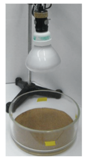
- Place the four small sponges around the perimeter of the arena, in alternating order of wet and dry, by leaning the sponges on the walls of the container at the base of the tape on the dishes (these sponges simulate hiding places for the isopods outdoors, such as logs). Does it matter if the sponges are equidistant from one another? (See Figure 1.)
- Adjust the 85W incandescent bulb about 20 cm vertically from the center of the arena (Figure 1). Record the temperature of the center of the arena with the light off, then turn on the lamp and record the temperature immediately. Your group may record the temperature of the center of the arena every minute during your 5-minute experiment.
- Release 20–24 isopods into the center of the arena. You will be performing a chi-square analysis on this data, so how many isopods should you use minimally? Record observations of isopod behavior in your lab notebook. Do the isopods tend to stay under a selected sponge or move around? You may want to record the number of isopods that are not under a sponge after each minute.
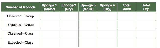
- After 5 minutes, count the number of isopods under each sponge and enter this information into your lab notebook in the format of Table 1.
- Sketch (or photograph) the arrangement and condition (moist or dry) of sponges in the arena.
- Complete the Data Analysis as a class.
Table 1 Data Table for Isopod Experiment: Moist Versus Dry Habitat Preferences
Pool (add) the number of isopods found under the moist sponges and the number under the dry sponges in your group experiment and enter these totals into the far right columns. Calculate the number of isopods expected in the different sites if the animals showed no habitat preference and distributed themselves evenly among microhabitats (total number isopods/total number of sites). Do the same calculations for class data.
2.7 Activity 2: Working with Continuous Data from Isopod Behavior Experiments
Purpose
These two experiments are designed as examples of experiments using continuous variables. Your lab class will repeat one or the other of the two experiments.
Learning Objectives
After successful completion of this activity, you should be able to:
LO49 Formulate a hypothesis
LO54 Set up and collect continuous data for an isopod behavior experiment
LO57 Organize data from an experiment in a way that allows you to search for patterns or trends
Materials
Isopod choice tube and delivery apparatus
Isopod arenas (Two 8′′ culture dishes with graph paper bottoms)
85W flood light on ring stand
Sponge habitats
Isopods (provided by students)
RO water
Transfer pipettes
Light meter (or use light meter app)
Vernier caliper
Permanent marker
Ruler and Vernier calipers
Thermometer, pH meter, and balance
2.8 Activity 2A: How Long Does It Take for an Isopod to Select One Treatment over Another in a Two-Choice Assay?
Activity 2A Procedure
- What is the specific scientific question you are asking and the null hypothesis associated with this experiment?
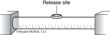
- Measure the length from the center of the choice tube chamber to each end where you will place treated or untreated sponges. Measure the temperature of the room.
- Obtain two small sponges and measure their L × W × H dimensions with a Vernier caliper. Use a 3 ml transfer pipette to moisten one of the sponges—3 ml of water on one side of the sponge and 3 ml of water on the other side of the sponge for a total of 6 ml of water. The sponge should be damp throughout. Measure the L × W × H dimensions of the sponge after it has been wet. Did the values change significantly? Avoid wetting the dry sponge.
- Gently place one isopod at the tube chamber release site (Figure 2) using the delivery apparatus provided. Once you are ready, release the isopod and start the timer.
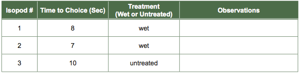
- As soon as the isopod passes the designated gradation of the choice tube chamber, stop the timer. Note the time and the treatment that the isopod chose (Table 2).
- Repeat the experiment with another isopod until you have tested 20 isopods minimally. Are the sample sizes used in this experiment sufficient for application of statistical analyses such as descriptive statistics or a t-test? Whenever you are planning to analyze data using descriptive statistics or t-tests, think about the role sample size will have on the validity of your analyses. Remember, data collected by each group in the class will serve as replicate data.
- Complete analysis of your group and class data.
Table 2 Isopod “Time to Choice” Experiment Data Collection Table
2.9 Activity 2B: How Does the Rate of Travel of Isopods Compare between Two Environments?
Activity 2B Procedure
- What is the specific scientific question you are asking and the null hypothesis associated with this experiment?
- Obtain two new culture dishes of the same size similar to that used in Activity 1. Place graph paper in the bottom of both arenas.
- Your class will select how it would like to designate its two environments. You might spritz the sides of one arena with water and leave the other arena dry. Alternatively, you might use one arena under room lighting and one under the 85W bulb, but keep both dry.
- Split your class in half—one half of the groups will treat every isopod tested to both environments (paired comparison), while the other groups will treat each isopod to one environment or the other but not both (unpaired comparison).
- Introduce one isopod to each environment and allow them to calm down for 1 minute. Observe isopod behavior at all times.
- Set your timer for 10 seconds. Observe both isopods and count the number of graph squares the individual isopods cross in the two arenas for the 10-second period. You may want to mark their starting point as soon as possible.
- Following the 10 seconds, if you are doing the paired scenario, switch the isopod in environment 1 with the isopod in environment 2 and vice versa. Repeat the experiment to collect data on each isopod in each environment (Table 3). If you are doing an unpaired scenario, remove the two isopods to the “used isopod” container and place a new isopod into each of the environments and repeat the experiment. The design of the experiment in a “paired” or “unpaired” configuration determines the type of statistical test you will apply to your data.
- Repeat the experiment for a total of 10 isopods if you are testing each isopod in both environments. Use a total of 20 isopods, 10 per environment, if you are testing each isopod in one environment only. Remember to allow each isopod 1 minute to calm down as soon as you place them in the culture dish.
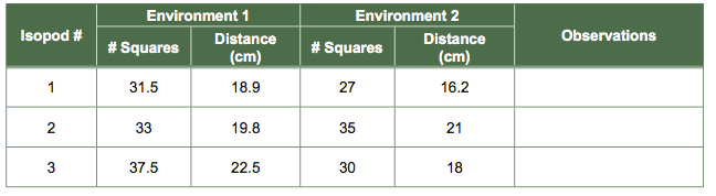
- Enter the number of graph squares crossed per isopod for your experiment and convert the distance covered to centimeters.
- Are the sample sizes used in this experiment sufficient for application of statistical analyses such as descriptive statistics or a t-test? Whenever you are planning to analyze data using descriptive statistics or t-tests, think about the role sample size will have on the validity of your analyses. Note: Data collected by each group that completed a similar experiment in the class can serve as replicate data.
Table 3 Isopod "Distance Traveled" Experiment Data Collection Table for Paired Data
2.10 Data Analysis: Analyzing Data Using Statistics
Part A: Describing Your Data
- What methods will you use to describe your class isopod data? Use the statistics flowchart on the back cover of your lab notebook. What analysis does it recommend?
- What descriptive characteristics of your class data can be calculated using the Excel Analysis Toolpak? Your instructor will assist you with this and you should insure that you understand the type of information that each of these descriptive characters provide and how they might be useful.
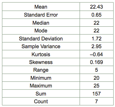
- Determine the mean, mode, median, standard error, and standard deviation of the class data for number of isopods that chose a wet habitat vs. a dry habitat. Repeat the analysis for the continuous isopod group data. The data should look similar to Table 4.
- What is the mean for each of the counts? How much variability is there for each of the counts? Does one environment produce more variability in isopod behavior than the other? If so, why do you think this is?
- If your group tested the amount of time required for an isopod to choose between one sponge treatment over another, what is the mean time for selection of dry sponge? Wet sponge? Does isopod choice for the untreated sponge show more variability than the water-treated sponge?
- If your group tested the rate of travel of isopods in two environments, what is the mean distance traveled in environment 1? Environment 2? Does isopod behavior in one environment show more variability than the other?
Table 4 Descriptive Statistics of Right Foot Lengths from BIO 204 Female Students
- As a class, prepare histograms of the compiled data for the “time to choice” for the untreated sponge and for the treated sponge if your class completed 2A. If your class completed 2B, produce histograms of the distances traveled for environment 1 and for environment 2. Histograms and frequency distributions are commonly applied to data to look for trends or patterns. What patterns do you notice when you compare the histograms for 2A data, “time to choice” between the untreated and treated sponge? What patterns do you notice when you compare histograms for 2B data, “distance traveled” between environment 1 versus environment 2?
2.11 Data Analysis: Analyzing Data Using Statistics Con't
Part B: Analyzing Categorical Data with the Chi-Square (Goodness of Fit) Test
Background
The isopod behavior experiment testing whether isopods choose wet or dry habits can be simplified to one comparison: Are the isopods randomly assorting into the microhabitats OR are the isopods distinguishing between the microhabitats and selecting them based on preference? We use statistics to test whether isopods are evenly distributed with respect to the different sites.
Analysis Is a Guessing Game without the Use of Statistics
We based our expected values on the null hypothesis, which states that the treatment had no effect on isopod behavior; thus, isopods should be distributed evenly with respect to the different microhabitats. For example, if there were 20 animals in our arena and two possible sites where they could hide, we would expect to find about 10 animals in each site if they showed no preference for the different habitats. However, if the animals display a preference for one site over another, we might observe an uneven distribution of isopods with respect to habitat. But how do we know if this distribution is meaningful and not due to random chance?
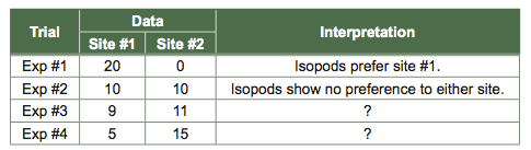
If all 20 isopods in the example above were found in one site and 0 were found in the second site, the isopods would be unevenly distributed, and we would conclude that they were displaying a habitat preference. Similarly, if 10 were found in one site and 10 at the second site, the isopods clearly would be evenly distributed, and we would conclude that they had no preference for the two microhabitats offered in the experiment. But what if we found 9 isopods at one site and 11 at another? Would we conclude this to be an equal or an unequal distribution with respect to microhabitat? What about 5 and 15? Do the results differ from the expected results simply due to chance, or due to the treatment effect that we were testing (e.g., wet vs. dry)? Statistics can help us with this question. But what statistical test should we use to analyze our data? Follow this series of questions to determine the right statistical test to select based on our data and experiment.
- What type of question are we asking for Activity 1? Did we compare averages, error, groups, or variables? For the Activity 1 isopod experiment, we studied distributions of isopods, or groups.
- What type of data are we collecting? Did we collect data that was continuous (e.g., length in meters), categorical (e.g., boy and girl), parametric (data are distributed as a bell curve), or circular (measured on a repeating scale; e.g., degrees on a compass)? In today’s lab, our data was the number of isopods under a particular sponge. This is an example of categorical data, which is data that can only be certain values or whole numbers. The isopods cannot be split into two and occupy multiple categories at the same time, nor can one isopod occupy a fraction of a category. We will address the other measurements you recorded during this lab after we address the categorical data.
- What type of comparison are we making? Did we compare our sample distribution to one other sample (binomial comparison), to multiple other samples, to a parent distribution, or to a null hypothesis? For this activity we conducted a binomial comparison (wet vs. dry).
- How many comparisons are we making? We are making one comparison between our data and the null hypothesis.
- Are our samples related? Are we independently collecting data or are our samples paired or grouped? The answer is that our data is independently collected. This is why it is important to select new isopods for each trial. If you used the same isopods for two trials, your data from both would be paired. If you used the same isopods over and over, then the samples would be grouped.
- What statistical test(s) should we use based on the answers to the previous questions and the statistics flowchart in your lab notebook—Chi-square or G-test?
Before we use any statistical test to analyze our data, we should always ask the following very important question: What are the assumptions of our statistical test?
Assumptions for Chi-Square:
- Your categorical data must be nominal and not ordinal. An example of ordinal data in which the categories are in order is stages of cancer, where the stages might be 1, 2, 3, etc. An example of nominal data in which the categories are NOT in order is male and female.
- Your sample size must be greater than five per category. If it isn’t, this test is inaccurate. This is why it was important to select more than 10 isopods if you used two categories.
Chi-Square Example (also refer to Appendix C and MathStats CatchUp Guide chapter 40):
Given the roughly 1:1 ratio of males and females in the human population, we might expect the number of males and females on a bus to be equal at any given time. Suppose we census a busload of people and find the following:

There seem to be many more females than males on the bus. But, is this deviation from a 1:1 ratio in the number of males to females due to chance or some other cause? To find out, we perform a chi-square test.
Calculating χ2: The general formula for calculating the χ2 statistic is as follows:
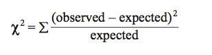
For each possible class (in our example there are two: males or females), you first calculate the difference between the observed and expected values and square this difference. You then divide this squared difference by the expected value, and then sum the values for all possible classes. The larger the difference between the observed and expected values, the larger the χ2 value. In our example:
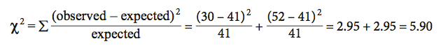
Calculating Probability: The calculated χ2 statistic for these data is 5.90. To determine the probability level (P value) for this test statistic, we first determine the degrees of freedom (d.f.) for the test, then look up the χ2 value in the probability table (Appendix C).
Degrees of Freedom (d.f.): The degrees of freedom are determined by the total number of classes minus 1. Because there are two classes in our example (males and females), the degree of freedom is 1 (# of classes – 1 = 2 – 1 = 1 d.f.).
P Values: To determine the probability associated with a givenχ2 statistic, look in the row of the table for the appropriate degrees of freedom (in our example, d.f. = 1, so you look in the first row) and look for your χ2 statistic. You will not find your exact χ2 value, but you can locate which columns, and therefore P values, match your results. If the P value is greater than 5% (to the left of the P = 0.05 column), you would conclude that the difference between the observed and expected results is due to chance. If the P value is less than 5% (to the right of the P = 0.05 column), then you conclude that the observed distribution is most likely not caused by chance, but rather is caused by some other effect.
Interpreting Statistical Results: For our bus-rider sample, (χ2 = 5.90), the number of classes is 2, so d.f. = 1 and we look in the first row of the table where 5.90 is found between P = 0.01 and P = 0.05. Thus, the probability that the difference between the observed and expected results is due to chance is very low, between 1% and 5% (0.01 < P < 0.05). Because P < 0.05, we can conclude that the greater number of females compared to males on the bus is not due to chance alone, but due to some other effect. In this example, we were not testing a specific treatment effect, so we don’t know the exact cause of the deviation from a 1:1 ratio. However, there may be many possible causes—for example, a Girl Scout Troop might have jumped on the bus just before we took the census.
2.12 Part B Procedure
- Each member of your group should analyze the data from the isopod activity 1 for both group and class data:
- State the specific predictions of the null hypothesis based on the number of isopods used in the experiment.
- Write the equation used to calculate the chi-square value.
- Show the chi-square equation with all of your values entered.
- Show the steps in solving the chi-square equation leading to the final chi-square value.
- State the degrees of freedom (d.f.) used. Show the calculation used to determine d.f.
- Determine the P value from the chi-square probability test table in Appendix C. You can also calculate the exact P value using Excel.
- Write a few sentences stating the conclusion of your experiment. Compare and contrast your group and class results.
- What additional data did you collect for your experiment? What type of data did you collect? Would you represent this data in tabular or graphical format to learn more about trends in your experiment? Would you apply statistical analyses to any of those data sets? If so, which test(s) and why? What other data could you have collected for this experiment? Explain.
- Turn in your data analysis to your lab instructor.
2.13 Part C: Testing for Possible Relationships between Variables
- How would you test whether there are associations between isopod body dimensions or weight and the rate at which they choose a treatment or the distance they traveled in a given environment, assuming the variables are independent of one another? Dependent on one another? Turn to the back page of your lab notebook to the statistics flowchart. What analysis does it recommend for each of these scenarios? Why does variable independence or dependence matter?
- You did not collect data on your isopods’ body dimensions or their weight in order to make these comparisons, but to demonstrate how to test for relationships using the data of isopod body length and width provided and the computer program Excel to determine if there is a correlation of isopod body length with width.
- Make a scatter plot of length and width in Excel. Does it matter which variable you place on the x-axis or y-axis for this statistical test?
- Determine the correlation coefficient “R” for the data set using the Excel function for correlation (correl). Based on the “R” values, were the isopod body dimensions strongly (> 0.6) or weakly correlated (< 0.4) with each other? Can you think of a case in which your data would not support known correlations in a body dimension study?
- Use Excel for linear regression analysis. Insert a regression line (trendline) in your scatter plot along with the slope equation and “R2” value. How well does the slope equation mathematically map your data? What does the “R2” value tell you about the residual error? For this test it matters what variable you place on the x-axis. This is the independent variable that can predict the value of a dependent variable. If, for example, you use isopod body length as your independent variable, you may be able to predict width, your dependent variable. For our purposes, you may arbitrarily select one variable to be the independent variable in your graph.
Remember: A high correlation suggests a relationship between two variables, but does not determine the cause and effect relationship. For this, you would have to know a great deal more about the nature of these relationships.
2.14 Data Analysis: Analyzing Data Using Statistics Con't
Part D: Comparing Means of Sample Populations
Purpose
Scientists very commonly compare means (averages) of independent data such as before and after, control and treatment, or changes over time of the same sample for data such as growth. When sample sizes are small, data means can be compared using a common kind of statistical test called a t-test. There are many times when we must make comparisons between means of data in which there is dependence between them—this comparison is called a paired t-test. An example of paired measurements are “before and after exercise” heart rate measurements on the same individual. However, the simplest t-test, called an unpaired t-test, is used to compare the means of independent samples. An example of independent samples would be average heart rates for two different individuals taken over the same period of time.
We will apply a t-test to our activity 2 data to compare the means between isopod “time to choice” for untreated sponge versus water-treated sponge. We will also compare the distance traveled in environment 1 versus environment 2. This leads to the questions, Do isopods move more quickly toward water-treated sponges over untreated sponges? Do isopods tend to travel longer distances in a dry habitat versus a moist habitat? Do isopods tend to travel longer distances in a well-lit habitat versus one that is not as well lit?
Refer to Blackboard for information about the t-test. Make sure you understand the rationale for comparing t-values and determining the critical t-value based on particular significance levels.
Part D Procedure
- State the hypothesis and the null hypothesis for your t-test comparison: “time to choice” for untreated to water-treated sponge, distance traveled in moist versus dry environment, or distance traveled in well-lit (i.e., with lamp) versus room-lit environment.
- What type of t-test, paired or unpaired, should you apply to your data? If you compared the same isopod from a sample population under two different conditions, then you should use a paired t-test. If you compared different isopods from a sample population under two different conditions, then you should apply an unpaired t-test.
- Assumption of Normality: Before you proceed with the t-test, you need to know if your data is normally distributed. Perform descriptive statistics of your data using Excel, then perform a simple check. If your data (the minimum and the maximum values) lie outside ± 2 standard deviations (SD) from your mean then it is not normally distributed. Would you expect your isopod data to be distributed normally?
- If the data is skewed, you need to transform it by adding a constant (e.g., the number 10) and take the log of each value. Excel will automatically do this transformation: type into a cell = log (data value + 10).
- Now we can quickly do the statistical analysis using the Data Analysis ToolPak in Excel: Data > Data Analysis > t-test. Which t-test function do you select? If the data is paired, select “Paired Two-Sample for Means.” If the data is unpaired and the variances are similar, select “Two-Sample Assuming Equal Variances”; otherwise select the choice for “Unequal Variances.”
- Your instructor will direct you in how to complete the analysis.
- Based on the results of your t-test, answer the following questions:
- What conclusion can you draw from your statistical analyses? Is there a difference between the two treatments with respect to “time to choice” or environments with respect to “distance traveled”?
- Did your t-test results support or reject your null hypothesis? Explain based on your critical t-value.
- Was there much variation for each data set? Explain.
- How strong were the correlations between data sets? Explain.
You will have an opportunity to repeat one of these studies next lab testing your own hypothesis. You should plan to bring in your own supplies if you want to make changes to the isopod arena design or choice tube chamber design (i.e., colored cellophane, filter paper, leaves, bark, etc.). You are welcome to bring in reagents that are innocuous to humans and isopods. It is recommended that you refer to the literature for background on isopods. If you have time at the end of this lab, discuss some questions with your group about isopod behavior that you would like to answer. Be creative with your experimental design. An isopod setup is present in the BLC to aid you with preparation.