Chapter . Impact 1.1
Impact…ON ENVIRONMENTAL SCIENCE I1.1: The gas laws and the weather
The biggest sample of gas readily accessible to us is the atmosphere, a mixture of gases with the composition summarized in Table I1.1. The composition is maintained moderately constant by diffusion and convection (winds, particularly the local turbulence called eddies) but the pressure and temperature vary with altitude and with the local conditions, particularly in the troposphere (the ‘sphere of change’), the layer extending up to about 11 km.
| Component | Percentage by volume | Percentage by mass |
|---|---|---|
| Nitrogen, N2 | 78.08 | 75.53 |
| Oxygen, O2 | 20.95 | 23.14 |
| Argon, Ar | 0.93 | 1.28 |
| Carbon dioxide, CO2 | 0.031 | 0.047 |
| Hydrogen, H2 | 5.0 × 10⁻³ | 2.0 × 10⁻⁴ |
| Neon, Ne | 1.8 × 10⁻³ | 1.3 × 10⁻³ |
| Helium, He | 5.2 × 10⁻⁴ | 7.2 × 10⁻⁵ |
| Methane, CH4 | 2.0 × 10⁻⁴ | 1.1 × 10⁻⁴ |
| Krypton, Kr | 1.1 ×10⁻⁴ | 3.2 × 10⁻⁴ |
| Nitric oxide, NO | 5.0 × 10⁻⁵ | 1.7 × 10⁻⁶ |
| Xenon, Xe | 8.7 × 10⁻⁶ | 1.2 × 10⁻⁵ |
| Ozone, O3; summer | 7.0 × 10⁻⁶ | 1.2 × 10⁻⁵ |
| Ozone, O3; winter | 2.0 × 10⁻⁶ | 3.3 × 10⁻⁶ |
In the troposphere the average temperature is 15 °C at sea level, falling to –57 °C at the bottom of the tropopause at 11 km. This variation is much less pronounced when expressed on the Kelvin scale, ranging from 288 K to 216 K, an average of 268 K. If we suppose that the temperature has its average value all the way up to the tropopause, then the pressure varies with altitude, h, according to the barometric formula:
p = p0e–h/H
where p0 is the pressure at sea level and H is a constant approximately equal to 8 km. More specifically, H = RT/Mg, where M is the average molar mass of air and T is the temperature. This formula represents the outcome of the competition between the potential energy of the molecules in the gravitational field of the Earth and the stirring effects of thermal motion; it is derived on the basis of the Boltzmann distribution (Foundations B). The barometric formula fits the observed pressure distribution quite well even for regions well above the troposphere (Fig. I1.1). It implies that the pressure of the air falls to half its sea-level value at h= H ln 2, or 6 km.
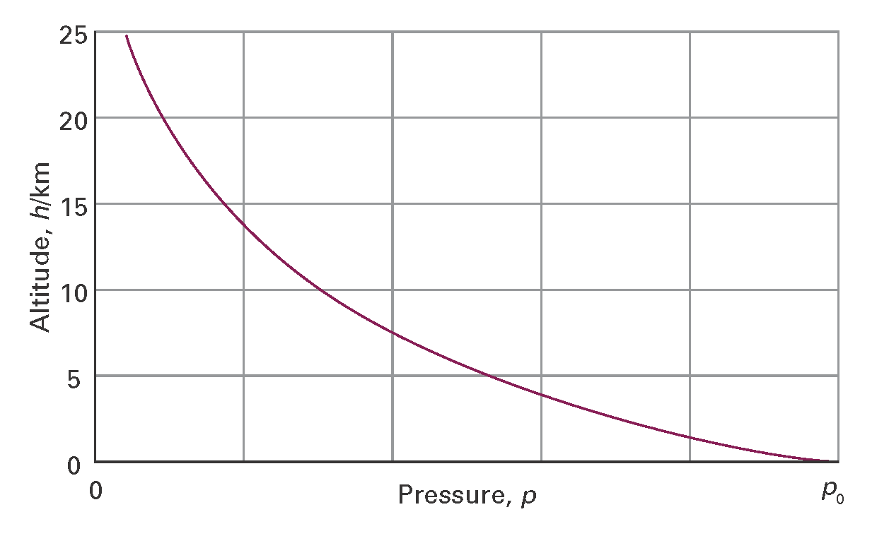
Figure I1.1 The variation of atmospheric pressure with altitude, as predicted by the barometric formula and as suggested by the ‘US Standard Atmosphere’, which takes into account the variation of temperature with altitude.
Local variations of pressure, temperature, and composition in the troposphere are manifest as ‘weather’. A small region of air is termed a parcel. First, we note that a parcel of warm air is less dense than the same parcel of cool air. As a parcel rises, it expands adiabatically (that is, without transfer of heat from its surroundings), so it cools. Cool air can absorb lower concentrations of water vapour than warm air, so the moisture forms clouds. Cloudy skies can therefore be associated with rising air and clear skies are often associated with descending air.
The motion of air in the upper altitudes may lead to an accumulation in some regions and a loss of molecules from other regions. The former result in the formation of regions of high pressure (‘highs’ or anticyclones) and the latter result in regions of low pressure (‘lows’, depressions, or cyclones). On a weather map, such as that shown in Fig. I1.2, the lines of constant pressure marked on it are called isobars. Elongated regions of high and low pressure are known, respectively, as ridges and troughs.
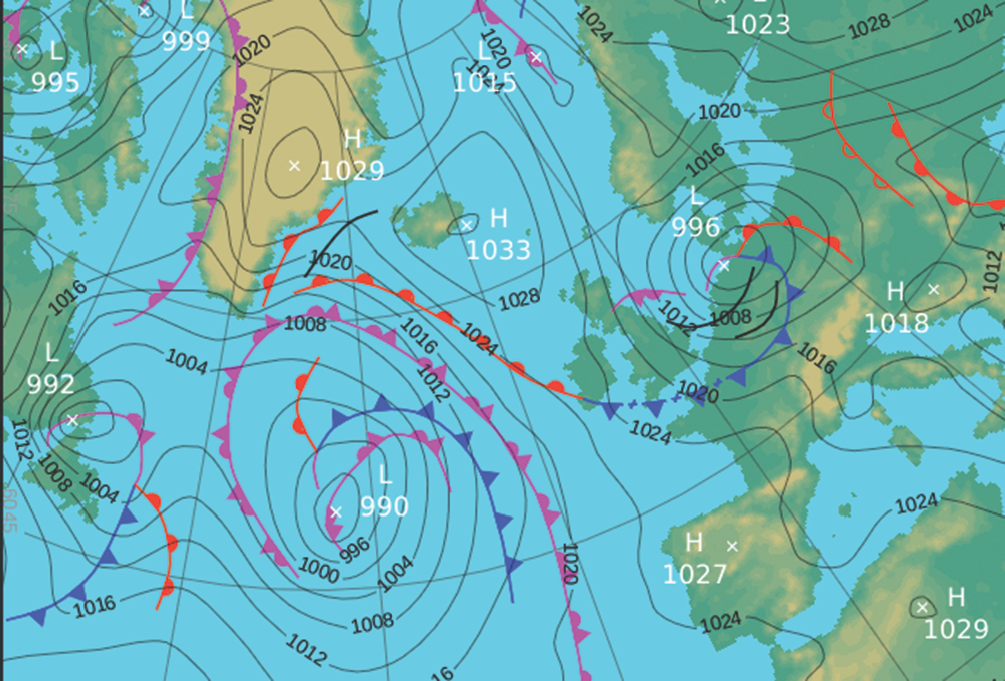
Figure I1.2 A typical weather map; in this case, for the North Atlantic and neighbouring regions on 10 December 2012. For current maps, go to your national weather service.
Horizontal pressure differentials result in the flow of air that we call wind (Fig. I1.3).Winds coming from the north in the northern hemisphere and from the south in the southern hemisphere are deflected towards the west as they migrate from a region where the Earth is rotating slowly (at the poles) to where it is rotating most rapidly (at the equator). Winds travel nearly parallel to the isobars, with low pressure to their left in the northern hemisphere and to the right in the southern hemisphere. At the surface, where wind speeds are lower, the winds tend to travel perpendicular to the isobars from high to low pressure. This differential motion results in a spiral outward flow of air clockwise in the northern hemisphere around a high and an inward anticlockwise flow around a low.
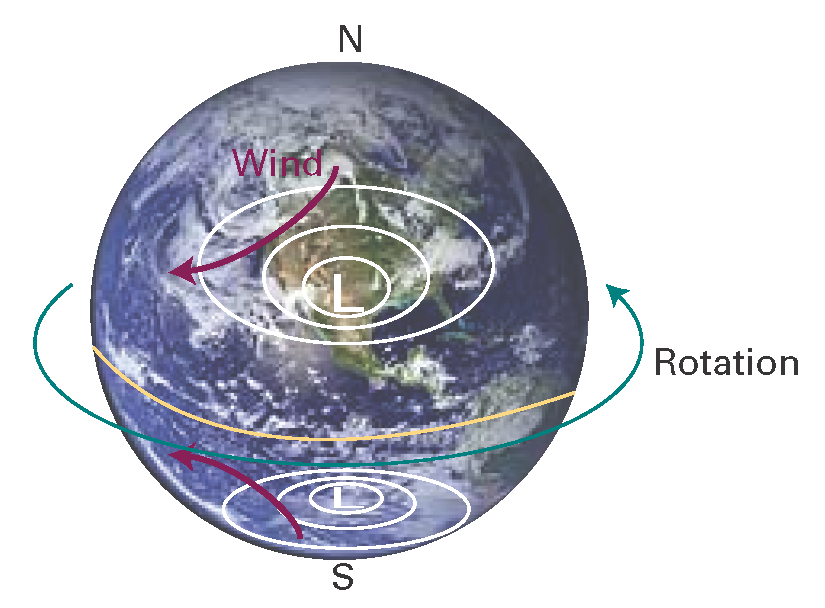
Figure I1.3 The flow of air (‘wind’) around regions of high and low pressure in the northern and southern hemispheres.
The air lost from regions of high pressure is restored as an influx of air converges into the region and descends. As we have seen, descending air is associated with clear skies. It also becomes warmer by compression as it descends, so regions of high pressure are associated with high surface temperatures. In winter, the cold surface air may prevent the complete fall of air, and result in a temperature inversion, with a layer of warm air over a layer of cold air. Geographical conditions may also trap cool air, as in Los Angeles, and the photochemical pollutants we know as smog may be trapped under the warm layer.