24.1 Quantitative Characteristics Vary Continuously and Many Are Influenced by Alleles at Multiple Loci
Qualitative, or discontinuous, characteristics possess only a few distinct phenotypes (Figure 24.1a); these characteristics are the types studied by Mendel (e.g., round and wrinkled peas) and have been the focus of our attention thus far. However, many characteristics vary continuously along a scale of measurement with many overlapping phenotypes (Figure 24.1b). They are referred to as continuous characteristics, and are also called quantitative characteristics because any individual’s phenotype must be described by a quantitative measurement. Examples of quantitative characteristics include height, weight, and blood pressure in humans, growth rate in mice, seed weight in plants, and milk production in cattle.
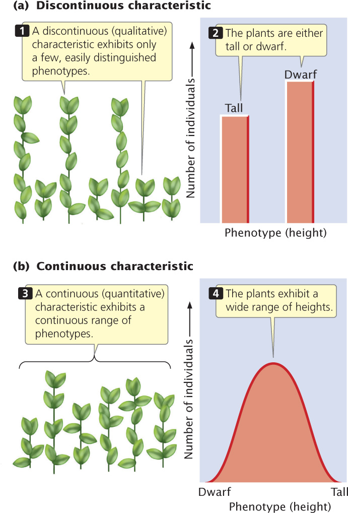
Quantitative characteristics arise from two phenomena. First, many are polygenic: they are influenced by genes at many loci. If many loci take part, many genotypes are possible, each producing a slightly different phenotype. Second, quantitative characteristics often arise when environmental factors affect the phenotype because environmental differences result in a single genotype producing a range of phenotypes. Most continuously varying characteristics are both polygenic and influenced by environmental factors, and these characteristics are said to be multifactorial.
The Relation Between Genotype and Phenotype
For some discontinuous characteristics, the relation between genotype and phenotype is straightforward. Each genotype produces a single phenotype, and most phenotypes are encoded by a single genotype. Dominance and epistasis may allow two or three genotypes to produce the same phenotype, but the relation remains simple. This simple relation between genotype and phenotype allowed Mendel to decipher the basic rules of inheritance from his crosses with pea plants; it also permits us both to predict the outcome of genetic crosses and to assign genotypes to individuals.
685
For quantitative characteristics, the relation between genotype and phenotype is often more complex. If the characteristic is polygenic, many different genotypes are possible, several of which may produce the same phenotype. For instance, consider a plant whose height is determined by three loci (A, B, and C), each of which has two alleles. Assume that one allele at each locus (A+, B+, and C+) encodes a plant hormone that causes the plant to grow 1 cm above its baseline height of 10 cm. The other allele at each locus (A−, B−, and C−) does not encode a plant hormone and thus does not contribute to additional height. If we consider only the two alleles at a single locus, 3 genotypes are possible (A+A+, A+A−, and A−A−). If all three loci are taken into account, there are a total of 33 = 27 possible multilocus genotypes (A+A+ B+B+ C+C+, A+A−B+B+ C+C+, etc.). Although there are 27 genotypes, they produce only seven phenotypes (10 cm, 11 cm, 12 cm, 13 cm, 14 cm, 15 cm, and 16 cm in height). Some of the genotypes produce the same phenotype (Table 24.1); for example, genotypes A+A− B−B− C−C−, A−A− B+B− C−C−, and A−A− B−B− C+C− all have one gene that encodes a plant hormone. Each of these genotypes produces one dose of the hormone and results in a plant that is 11 cm tall. Even in this simple example of only three loci, the relation between genotype and phenotype is quite complex. The more loci encoding a characteristic, the greater the complexity. As the number of loci encoding a characteristic increases, the number of potential phenotypes increases, and differences between individual phenotypes becomes more difficult to distinguish.
| Plant Genotype | Doses of Hormone | Height (cm) |
|---|---|---|
| A−A− B−B− C−C− | 0 | 10 |
| A+A− B−B− C−C− | 1 | 11 |
| A−A− B+B− C−C− | ||
| A−A− B−B− C−C+ | ||
| A+A+ B−B− C−C− | 2 | 12 |
| A−A− B+B+ C−C− | ||
| A−A− B−B− C+C+ | ||
| A+A− B+B− C−C− | ||
| A+A− B−B− C+C− | ||
| A−A− B+B− C+C− | ||
| A+A+ B+B− C−C− | 3 | 13 |
| A+A+ B−B− C+C− | ||
| A+A− B+B+ C−C− | ||
| A−A− B+B+ C+C− | ||
| A+A− B−B− C+C+ | ||
| A−A− B+B− C+C+ | ||
| A+A− B+B− C+C− | ||
| A+A+ B+B+ C−C− | 4 | 14 |
| A+A+ B+B− C+C− | ||
| A+A− B+B+ C+C− | ||
| A−A− B+B+ C+C+ | ||
| A+A+ B−B− C+C+ | ||
| A+A− B+B− C+C+ | ||
| A+A+ B+B+ C+C− | 5 | 15 |
| A+A− B+B+ C+C+ | ||
| A+A+ B+B− C+C+ | ||
| A+A+ B+B+ C+C+ | 6 | 16 |
| Note: Each + allele contributes 1 cm In height above a baseline of 10 cm. | ||
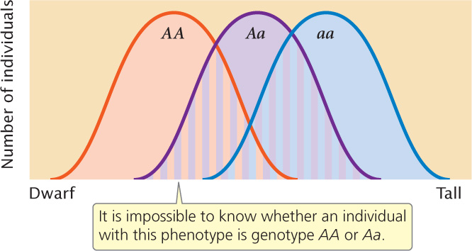
The influence of environment on a characteristic also can complicate the relation between genotype and phenotype. Because of environmental effects, the same genotype can produce a range of potential phenotypes. The phenotypic ranges of different genotypes can overlap, making it difficult to know whether individuals differ in phenotype because of genetic or environmental differences (Figure 24.2).
In summary, the simple relation between genotype and phenotype that exists for many qualitative (discontinuous) characteristics is absent for quantitative characteristics, and it is impossible to assign a genotype to an individual on the basis of its phenotype alone. The methods used for analyzing qualitative characteristics (examining the phenotypic ratios of progeny from a genetic cross) will not work for quantitative characteristics. Our goal remains the same: we wish to make predictions about the phenotypes of offspring produced in a genetic cross. We may also want to know how much of the variation of a characteristic results from genetic differences and how much results from environmental differences. To answer these questions, we must turn to statistical methods that allow us to make predictions about the inheritance of phenotypes in the absence of information about the underlying genotypes. ![]() TRY PROBLEM 16
TRY PROBLEM 16
686
Types of Quantitative Characteristics
Before we look more closely at polygenic characteristics and relevant statistical methods, we need to more clearly define what is meant by a quantitative characteristic. Thus far, we have considered only quantitative characteristics that vary continuously in a population. A continuous characteristic can theoretically assume any value between two extremes; the number of phenotypes is limited only by our ability to precisely measure the phenotype. Human height is a continuous characteristic because, within certain limits, people can theoretically have any height. Although the number of phenotypes possible with a continuous characteristic is infinite, we often group similar phenotypes together for convenience; we may say that two people are both 5 feet 11 inches tall, but careful measurement may show that one is slightly taller than the other.
Some characteristics are not continuous but are nevertheless considered quantitative because they are determined by multiple genetic and environmental factors. Meristic characteristics, for instance, are measured in whole numbers. An example is litter size: a female mouse can have 4, 5, or 6 pups but not 4.13 pups. A meristic characteristic has a limited number of distinct phenotypes, but the underlying determination of the characteristic can still be quantitative. These characteristics must therefore be analyzed with the same techniques that we use to study continuous quantitative characteristics.
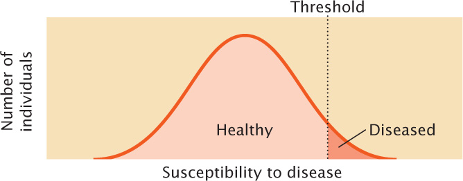
Another type of quantitative characteristic is a threshold characteristic, which is simply present or absent. Although threshold characteristics exhibit only two phenotypes, they are considered quantitative because they, too, are determined by multiple genetic and environmental factors. The expression of the characteristic depends on an underlying susceptibility (usually referred to as liability or risk) that varies continuously. When the susceptibility is larger than a threshold value, a specific trait is expressed (Figure 24.3). Diseases are often threshold characteristics because many factors, both genetic and environmental, contribute to disease susceptibility. If enough of the susceptibility factors are present, the disease develops; otherwise, it is absent. Although we focus on the genetics of continuous characteristics in this chapter, the same principles apply to many meristic and threshold characteristics.
Just because a characteristic can be measured on a continuous scale does not mean that it exhibits quantitative variation. One of the characteristics studied by Mendel was height of the pea plant, which can be described by measuring the length of the plant’s stem. However, Mendel’s particular plants exhibited only two distinct phenotypes (some were tall and others short), and these differences were determined by alleles at a single locus. The differences that Mendel studied were therefore discontinuous in nature.
CONCEPTS
Characteristics for which the phenotypes vary continuously are called quantitative characteristics. For most quantitative characteristics, the relation between genotype and phenotype is complex. Some characteristics for which the phenotypes do not vary continuously also are considered quantitative because they are influenced by multiple genes and environmental factors.
Polygenic Inheritance
After the rediscovery of Mendel’s work in 1900, questions soon arose about the inheritance of continuously varying characteristics. These characteristics had already been the focus of a group of biologists and statisticians, led by Francis Galton, who used statistical procedures to examine the inheritance of quantitative characteristics such as human height and intelligence. The results of these studies showed that quantitative characteristics were at least partly inherited, although the mechanism of inheritance was not yet known. Some biometricians argued that the inheritance of quantitative characteristics could not be explained by Mendelian principles, whereas others felt that Mendel’s principles acting on numerous genes (polygenes) could adequately account for the inheritance of quantitative characteristics.
This conflict began to be resolved by the work of Wilhelm Johannsen, who showed that continuous variation in the weight of beans was influenced by both genetic and environmental factors. George Udny Yule, a mathematician, proposed in 1906 that several genes acting together could produce continuous characteristics. This hypothesis was later confirmed by Herman Nilsson-Ehle, working on wheat and tobacco, and by Edward East, working on corn. The argument was finally laid to rest in 1918, when Ronald Fisher demonstrated that the inheritance of quantitative characteristics could indeed be explained by the cumulative effects of many genes, each following Mendel’s rules.
687
Kernel Color in Wheat
To illustrate how multiple genes acting on a characteristic can produce a continuous range of phenotypes, let us examine one of the first demonstrations of polygenic inheritance. Nilsson-Ehle studied kernel color in wheat and found that the intensity of red pigmentation was determined by three unlinked loci, each of which had two alleles.
Nilsson-Ehle’s Cross
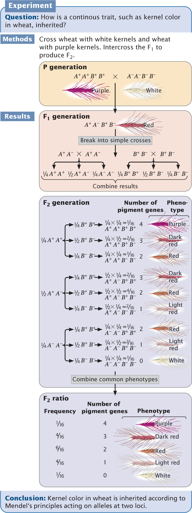
Nilsson-Ehle obtained several homozygous varieties of wheat that differed in color. Like Mendel, he performed crosses between these homozygous varieties and studied the ratios of phenotypes in the progeny. In one experiment, he crossed a variety of wheat that possessed white kernels with a variety that possessed purple (very dark red) kernels and obtained the following results:
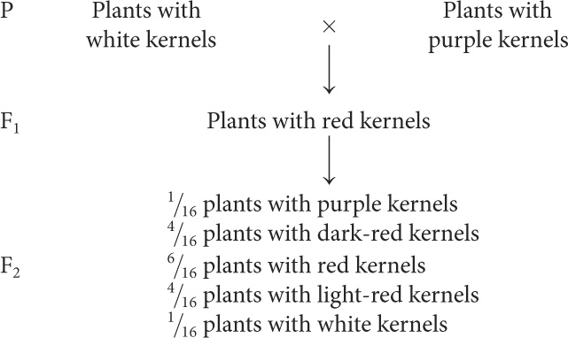
Interpretation of the Cross
Nilsson-Ehle interpreted this phenotypic ratio as the result of the segregation of alleles at two loci (although he found alleles at three loci that affect kernel color, the two varieties used in this cross differed at only two of the loci). He proposed that there were two alleles at each locus: one that produced red pigment and another that produced no pigment. We’ll designate the alleles that encoded pigment A+ and B+ and the alleles that encoded no pigment A− and B−. Nilsson-Ehle recognized that the effects of the genes were additive. Each gene seemed to contribute equally to color; so the overall phenotype could be determined by adding the effects of all the genes, as shown in the following table.
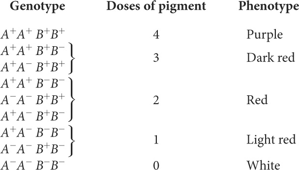
Notice that the purple and white phenotypes are each encoded by a single genotype, but other phenotypes may result from several different genotypes.
From these results, we see that five phenotypes are possible when alleles at two loci influence the phenotype and the effects of the genes are additive. When alleles at more than two loci influence the phenotype, more phenotypes are possible, and the color would appear to vary continuously between white and purple. If environmental factors had influenced the characteristic, individuals of the same genotype would vary somewhat in color, making it even more difficult to distinguish between discrete phenotypic classes. Luckily, environment played little role in determining kernel color in Nilsson-Ehle’s crosses, and only a few loci encoded color; so Nilsson-Ehle was able to distinguish among the different phenotypic classes. This ability allowed him to see the Mendelian nature of the characteristic.
Let’s now see how Mendel’s principles explain the ratio obtained by Nilsson-Ehle in his F2 progeny. Remember that Nilsson-Ehle crossed the homozygous purple variety (A+A+ B+B+) with the homozygous white variety (A−A− B−B−), producing F1 progeny that were heterozygous at both loci (A+A− B+B−). This is a dihybrid cross, like those that we worked in Chapter 3 except that both loci encode the same trait. All the F1 plants possessed two pigment-producing alleles that allowed two doses of color to make red kernels. The types and proportions of progeny expected in the F2 can be found by applying Mendel’s principles of segregation and independent assortment.
Let’s first examine the effects of each locus separately. At the first locus, two heterozygous F1s are crossed (A+A− × A+A−). As we learned in Chapter 3, when two heterozygotes are crossed, we expect progeny in the proportions  A+A+,
A+A+,  A+A−, and
A−A−. At the second locus, two heterozygotes also are crossed, and, again, we expect progeny in the proportions
B+B+,
B+B−, and
B−B−.
A+A−, and
A−A−. At the second locus, two heterozygotes also are crossed, and, again, we expect progeny in the proportions
B+B+,
B+B−, and
B−B−.
To obtain the probability of combinations of genes at both loci, we must use the multiplication rule of probability (see Chapter 3), the use of which assumes Mendel’s principle of independent assortment. The expected proportion of F2 progeny with genotype A+A+ B+B+ is the product of the probability of obtaining genotype A+A+ (
) and the probability of obtaining genotype B+B+ (
), or
×
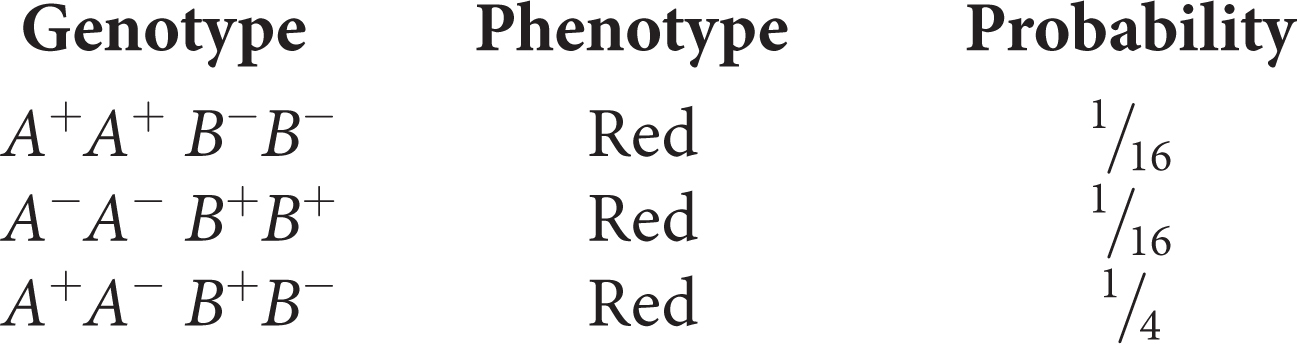
=  (Figure 24.4). The probabilities of each of the phenotypes can then be obtained by adding the probabilities of all the genotypes that produce that phenotype. For example, the red phenotype is produced by three genotypes:
688
Thus, the overall probability of obtaining red kernels in the F2 progeny is
+
+
=  . Figure 24.4 shows that the phenotypic ratio expected in the F2 is
purple,
. Figure 24.4 shows that the phenotypic ratio expected in the F2 is
purple,  dark red,
red,
light red, and
white. This phenotypic ratio is precisely what Nilsson-Ehle observed in his F2 progeny, demonstrating that the inheritance of a continuously varying characteristic such as kernel color is indeed according to Mendel’s basic principles.
dark red,
red,
light red, and
white. This phenotypic ratio is precisely what Nilsson-Ehle observed in his F2 progeny, demonstrating that the inheritance of a continuously varying characteristic such as kernel color is indeed according to Mendel’s basic principles.
Conclusions and Implications
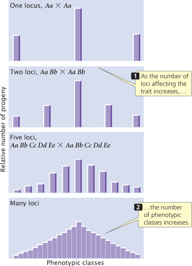
Nilsson-Ehle’s crosses demonstrated that the difference between the inheritance of genes influencing quantitative characteristics and the inheritance of genes influencing discontinuous characteristics is in the number of loci that determine the characteristic. When multiple loci affect a characteristic, more genotypes are possible, so the relation between the genotype and the phenotype is less obvious. As the number of loci affecting a characteristic increases, the number of phenotypic classes in the F2 increases (Figure 24.5).
Several conditions of Nilsson-Ehle’s crosses greatly simplified the polygenic inheritance of kernel color and made it possible for him to recognize the Mendelian nature of the characteristic. First, genes affecting color segregated at only two or three loci. If genes at many loci had been segregating, he would have had difficulty in distinguishing the phenotypic classes. Second, the genes affecting kernel color had strictly additive effects, making the relation between genotype and phenotype simple. Third, environment played almost no role in the phenotype; had environmental factors modified the phenotypes, distinguishing between the five phenotypic classes would have been difficult. Finally, the loci that Nilsson-Ehle studied were not linked, so the genes assorted independently. Nilsson-Ehle was fortunate: for many polygenic characteristics, these simplifying conditions are not present and Mendelian inheritance of these characteristics is not obvious. ![]() TRY PROBLEM 17
TRY PROBLEM 17
Determining Gene Number for a Polygenic Characteristic
The proportion of F2 individuals that resemble one of the original parents can be used to estimate the number of genes affecting a polygenic trait. When two individuals homozygous for different alleles at a single locus are crossed (A1A1 × A2A2) and the resulting F1 are interbred (A1A2 × A1A2), one-fourth of the F2 should be homozygous like each of the original parents. If the original parents are homozygous for different alleles at two loci, as are those in Nilsson-Ehle’s crosses, then
×
=
of the F2 should resemble one of the original homozygous parents. Generally, (
)n will be the proportion of individuals in the F2 progeny that should resemble each of the original homozygous parents, where n equals the number of loci with a segregating pair of alleles that affects the characteristic. This equation provides us with a possible means of determining the number of loci influencing a quantitative characteristic.
689
To illustrate the use of this equation, assume that we cross two different homozygous varieties of pea plants that differ in height by 16 cm, interbreed the F1, and find that approximately  of the F2 are similar to one of the original homozygous parental varieties. This outcome would suggest that four loci with segregating pairs of alleles (
= (
)4) are responsible for the height difference between the two varieties. Because the two homozygous strains differ in height by 16 cm and there are four loci each of which has two alleles (eight alleles in all), each of the alleles contributes 16 cm/8 = 2 cm in height.
of the F2 are similar to one of the original homozygous parental varieties. This outcome would suggest that four loci with segregating pairs of alleles (
= (
)4) are responsible for the height difference between the two varieties. Because the two homozygous strains differ in height by 16 cm and there are four loci each of which has two alleles (eight alleles in all), each of the alleles contributes 16 cm/8 = 2 cm in height.
This method for determining the number of loci affecting phenotypic differences requires the use of homozygous strains, which may be difficult to obtain in some organisms. It also assumes that all the genes influencing the characteristic have equal effects, that their effects are additive, and that the loci are unlinked. For many polygenic characteristics, these assumptions are not valid, and so this method of determining the number of genes affecting a characteristic has limited application. ![]() TRY PROBLEM 19
TRY PROBLEM 19
CONCEPTS
The same principles determine the inheritance of quantitative and discontinuous characteristics, but more genes take part in the determination of quantitative characteristics.
 CONCEPT CHECK 1
Briefly explain how the number of genes influencing a polygenic trait can be determined.