24.2 Statistical Methods Are Required for Analyzing Quantitative Characteristics
Because quantitative characteristics are described by a measurement and are influenced by multiple factors, their inheritance must be analyzed statistically. This section will explain the basic concepts of statistics that are used to analyze quantitative characteristics.
Distributions
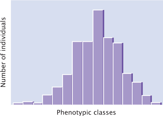
Understanding the genetic basis of any characteristic begins with a description of the numbers and kinds of phenotypes present in a group of individuals. Phenotypic variation in a group can be conveniently represented by a frequency distribution, which is a graph of the frequencies (numbers or proportions) of the different phenotypes (Figure 24.6). In a typical frequency distribution, the phenotypic classes are plotted on the horizontal (x) axis, and the numbers (or proportions) of individuals in each class are plotted on the vertical (y) axis. A frequency distribution is a concise method of summarizing all phenotypes of a quantitative characteristic.
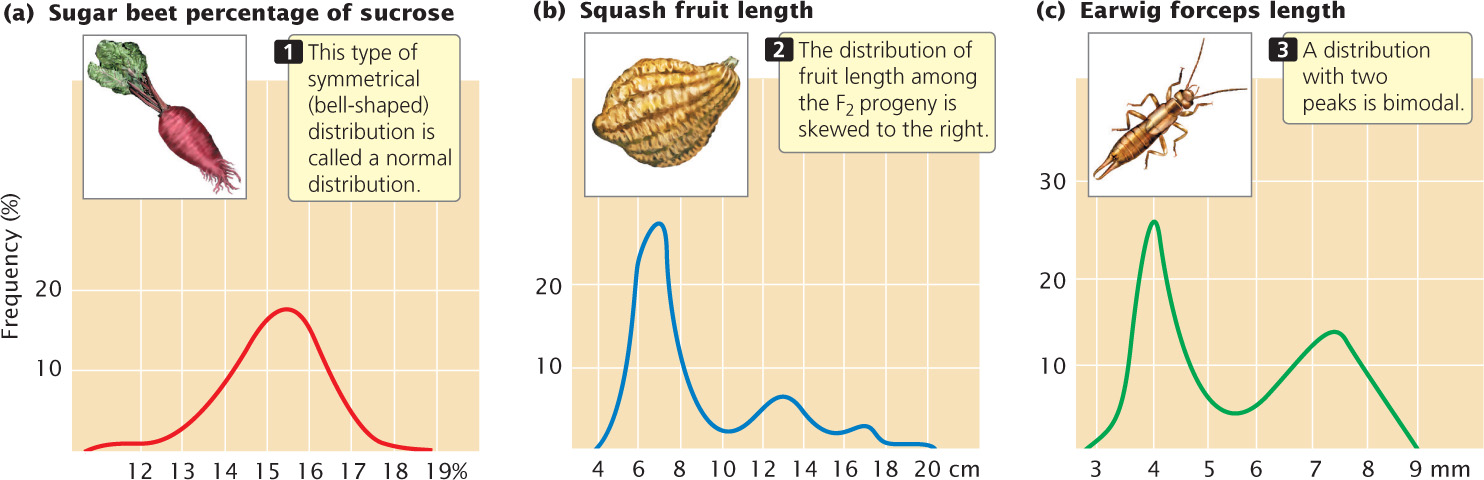
Connecting the points of a frequency distribution with a line creates a curve that is characteristic of the distribution. Many quantitative characteristics exhibit a symmetrical (bell-shaped) curve called a normal distribution (Figure 24.7a). Normal distributions arise when a large number of independent factors contribute to a measurement, as is often the case in quantitative characteristics. Two other common types of distributions (skewed and bimodal) are illustrated in Figure 24.7b and c.
690
Samples and Populations
Biologists frequently need to describe the distribution of phenotypes exhibited by a group of individuals. We might want to describe the height of students at the University of Texas (UT), but UT has more than 40,000 students and measuring all of them is not practical. Scientists are constantly confronted with this problem: the group of interest, called the population, is too large for a complete census. One solution is to measure a smaller collection of individuals, called a sample, and use those measurements to describe the population.
To provide an accurate description of the population, a good sample must have several characteristics. First, it must be representative of the whole population—for instance, if our sample consisted entirely of members of the UT basketball team we would probably overestimate the true height of the students. One way to ensure that a sample is representative of the population is to select the members of the sample randomly. Second, the sample must be large enough that chance differences between individuals in the sample and the overall population do not distort the estimate of the population measurements. If we measured only three students at UT and just by chance all three were short, we would underestimate the true height of the student population. Statistics can provide information about how much confidence to have in estimates based on random samples.
CONCEPTS
In statistics, the population is the group of interest; a sample is a subset of the population. The sample should be representative of the population and large enough to minimize chance differences between the population and the sample.
 CONCEPT CHECK 2
A geneticist is interested in whether asthma is caused by a mutation in the DS112 gene. the geneticist collects DNA from 120 people with asthma and 100 healthy people, and sequences the DNA. She finds that 35 of the people with asthma and none of the healthy people have a mutation in the DS112 gene. What is the population in this study?
- the 120 people with asthma.
- the 100 healthy people.
- the 35 people with a mutation in their gene.
- All people with asthma.
The Mean
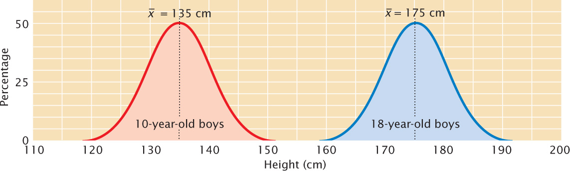
The mean, also called the average, provides information about the center of the distribution. If we measured the heights of 10-year-old and 18-year-old boys and plotted a frequency distribution for each group, we would find that both distributions are normal, but the two distributions would be centered at different heights, and this difference would be indicated in their different means (Figure 24.8).
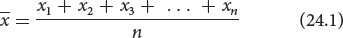
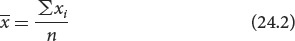
Suppose that we have five measurements of height in centimeters: 160, 161, 167, 164, and 165. If we represent a group of measurements as x1, x2, x3, and so forth, then the mean  is calculated by adding all the individual measurements and dividing by the total number of measurements in the sample (n):
In our example, x1 = 160, x2 = 161, x3 = 167, and so forth. The mean height
equals:

691
A shorthand way to represent this formula is
or
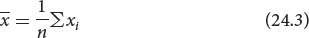
where the symbol Σ means “the summation of” and xi represents individual x values.
The Variance and Standard Deviation
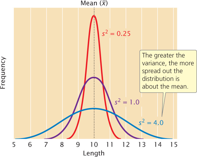
A statistic that provides key information about a distribution is the variance, which indicates the variability of a group of measurements, or how spread out the distribution is. Distributions can have the same mean but different variances (Figure 24.9). The larger the variance, the greater the spread of measurements in a distribution about its mean.
The variance (s2) is defined as the average squared deviation from the mean:

To calculate the variance, we (1) subtract the mean from each measurement and square the value obtained, (2) add all the squared deviations, and (3) divide this sum by the number of original measurements minus 1.
Another statistic that is closely related to the variance is the standard deviation (s), which is defined as the square root of the variance:

Whereas the variance is expressed in units squared, the standard deviation is in the same units as the original measurements; so the standard deviation is often preferred for describing the variability of a measurement.
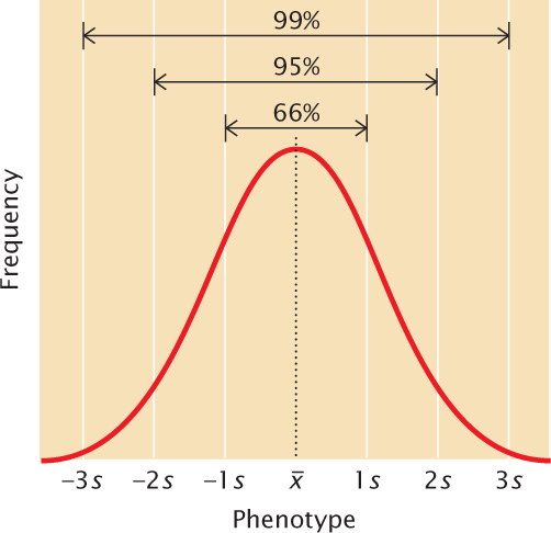
A normal distribution is symmetrical; so the mean and standard deviation are sufficient to describe its shape. The mean plus or minus one standard deviation ( ± s) includes approximately 66% of the measurements in a normal distribution; the mean plus or minus two standard deviations (
± 2s) includes approximately 95% of the measurements, and the mean plus or minus three standard deviations (
± 3s) includes approximately 99% of the measurements (Figure 24.10). Thus, only 1% of a normally distributed population lies outside the range of (
± 3s).
± s) includes approximately 66% of the measurements in a normal distribution; the mean plus or minus two standard deviations (
± 2s) includes approximately 95% of the measurements, and the mean plus or minus three standard deviations (
± 3s) includes approximately 99% of the measurements (Figure 24.10). Thus, only 1% of a normally distributed population lies outside the range of (
± 3s). ![]() TRY PROBLEM 22
TRY PROBLEM 22
692
CONCEPTS
The mean and the variance describe a distribution of measurements: the mean provides information about the location of the center of a distribution, and the variance provides information about its variability.
CONCEPT CHECK 3
The measurements of a distribution with a higher________will be more spread out.
- mean
- variance
- standard deviation
- variance and standard deviation
Correlation
The mean and the variance can be used to describe an individual characteristic, but geneticists are frequently interested in more than one characteristic. Often, two or more characteristics vary together. For instance, both the number and the weight of eggs produced by hens are important to the poultry industry. These two characteristics are not independent of each other. There is an inverse relation between egg number and weight: hens that lay more eggs produce smaller eggs. This kind of relation between two characteristics is called a correlation. When two characteristics are correlated, a change in one characteristic is likely to be associated with a change in the other.
Correlations between characteristics are measured by a correlation coefficient (designated r), which measures the strength of their association. Consider two characteristics, such as human height (x) and arm length (y). To determine how these characteristics are correlated, we first obtain the covariance (cov) of x and y:
The covariance is computed by (1) taking an x value for an individual and subtracting it from the mean of x
; (2) taking the y value for the same individual and subtracting it from the mean of y ; (3) multiplying the results of these two subtractions; (4) adding the results for all the xy pairs; and (5) dividing this sum by n − 1 (where n equals the number of xy pairs).
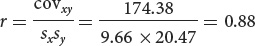
The correlation coefficient (r) is obtained by dividing the covariance of x and y by the product of the standard deviations of x and y:
A correlation coefficient can theoretically range from −1 to +1. A positive value indicates that there is a direct association between the variables (Figure 24.11a): as one variable increases, the other variable also tends to increase. A positive correlation exists for human height and weight: tall people tend to weigh more. A negative correlation coefficient indicates that there is an inverse relation between the two variables (Figure 24.11b): as one variable increases, the other tends to decrease (as is the case for egg number and egg weight in chickens).
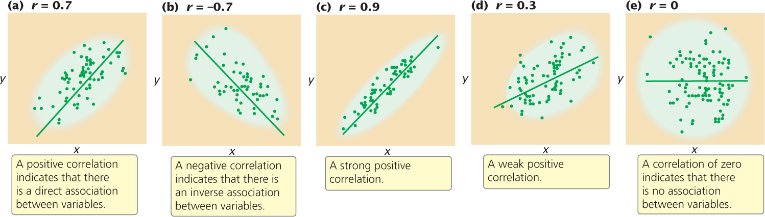
The absolute value of the correlation coefficient (the size of the coefficient, ignoring its sign) provides information about the strength of association between the variables. A coefficient of −1 or +1 indicates a perfect correlation between the variables, meaning that a change in x is always accompanied by a proportional change in y. Correlation coefficients close to −1 or close to +1 indicate a strong association between the variables: a change in x is almost always associated with a proportional increase in y, as seen in Figure 24.11c. On the other hand, a correlation coefficient closer to 0 indicates a weak correlation: a change in x is associated with a change in y but not always (Figure 24.11d). A correlation of 0 indicates that there is no association between variables (Figure 24.11e).
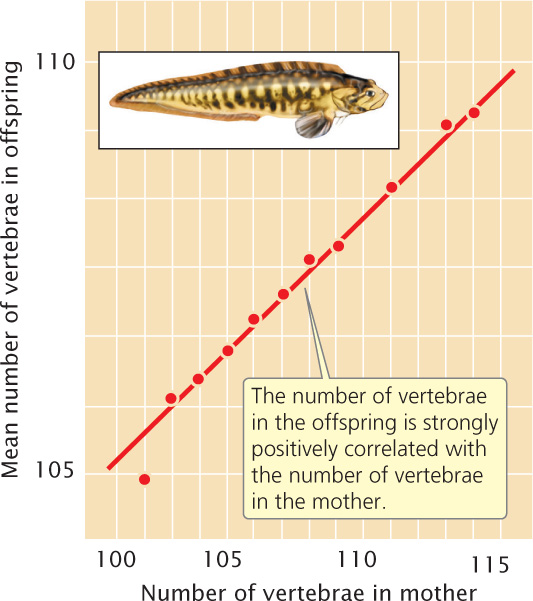
A correlation coefficient can be computed for two variables measured for the same individual, such as height (x) and weight (y). A correlation coefficient can also be computed for a single variable measured for pairs of individuals. For example, we can calculate for fish the correlation between the number of vertebrae of a parent (x) and the number of vertebrae of its offspring (y), as shown in Figure 24.12. This approach is often used in quantitative genetics.
693
A correlation between two variables indicates only that the variables are associated; it does not imply a cause-and-effect relation. Correlation also does not mean that the values of two variables are the same; it means only that a change in one variable is associated with a proportional change in the other variable. For example, the x and y variables in the following list are almost perfectly correlated, with a correlation coefficient of 0.99.
| x value | y value | |
|---|---|---|
| 12 | 123 | |
| 14 | 140 | |
| 10 | 110 | |
| 6 | 61 | |
| 3 | 32 | |
| Average: | 9 | 90 |
A high correlation is found between these x and y variables; larger values of x are always associated with larger values of y. Note that the y values are about 10 times as large as the corresponding x values; so, although x and y are correlated, they are not identical. The distinction between correlation and identity becomes important when we consider the effects of heredity and environment on the correlation of characteristics. ![]() TRY PROBLEM 25
TRY PROBLEM 25
Regression
Correlation provides information only about the strength and direction of association between variables. However, we often want to know more than just whether two variables are associated; we want to be able to predict the value of one variable given a value of the other.
A positive correlation exists between the body weight of parents and the body weight of their offspring; this correlation exists in part because genes influence body weight, and parents and children have genes in common. Because of this association between parental and offspring phenotypes, we can predict the weight of an individual on the basis of the weights of its parents. This type of statistical prediction is called regression. This technique plays an important role in quantitative genetics because it allows us to predict the characteristics of offspring from a given mating, even without knowledge of the genotypes that encode the characteristics.
Regression can be understood by plotting a series of x and y values. Figure 24.13 illustrates the relation between the weight of a father (x) and the weight of his son (y). Each father–son pair is represented by a point on the graph. The overall relation between these two variables is depicted by the regression line, which is the line that best fits all the points on the graph (deviations of the points from the line are minimized). The regression line defines the relation between the x and y variables and can be represented by

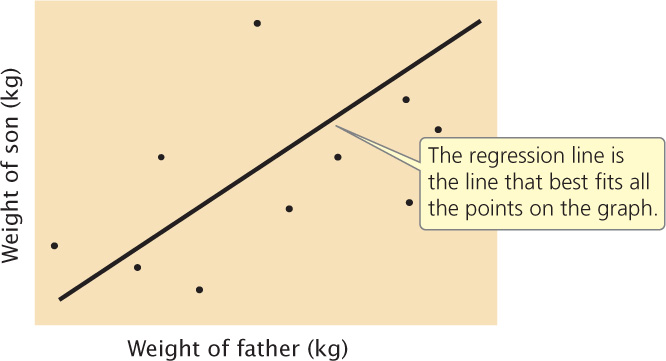
In Equation 24.8, x and y represent the x and y variables (in this case, the father’s weight and the son’s weight, respectively). The variable a is the y intercept of the line, which is the expected value of y when x is 0. Variable b is the slope of the regression line, also called the regression coefficient.
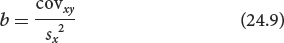
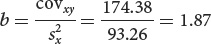
Trying to position a regression line by eye is not only very difficult but also inaccurate when there are many points scattered over a wide area. Fortunately, the regression coefficient and the y intercept can be obtained mathematically. The regression coefficient (b) can be computed from the covariance of x and y (covxy) and the variance of x (s) by
694
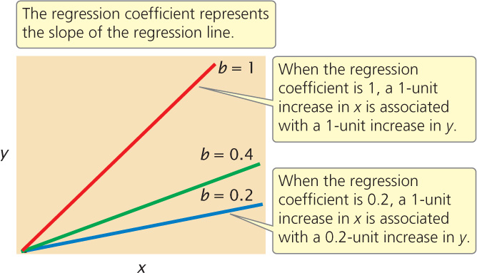
The regression coefficient indicates how much y increases, on average, per increase in x. Several regression lines with different regression coefficients are illustrated in Figure 24.14. Notice that as the regression coefficient increases, the slope of the regression line increases.
After the regression coefficient has been calculated, the y intercept can be calculated by substituting the regression coefficient and the mean values of x and y into the following equation:

The regression equation (y = a + bx, Equation 24.8) can then be used to predict the value of any y given the value of x.
CONCEPTS
A correlation coefficient measures the strength of association between two variables. The sign (positive or negative) indicates the direction of the correlation; the absolute value measures the strength of the association. Regression is used to predict the value of one variable on the basis of the value of a correlated variable.
CONCEPT CHECK 4
In Lubbock, texas, rainfall and temperature exhibit a significant correlation of −0.7. Which conclusion is correct?
- There is usually more rainfall when the temperature is high.
- There is usually more rainfall when the temperature is low.
- Rainfall is equally likely when the temperature is high or low.
WORKED PROBLEMS
Body weights of 11 female fishes and the numbers of eggs that they produce are:
| Weight (mg) | Eggs (thousands) |
|---|---|
| x | y |
| 14 | 61 |
| 17 | 37 |
| 24 | 65 |
| 25 | 69 |
| 27 | 54 |
| 33 | 93 |
| 34 | 87 |
| 37 | 89 |
| 40 | 100 |
| 41 | 90 |
| 42 | 97 |
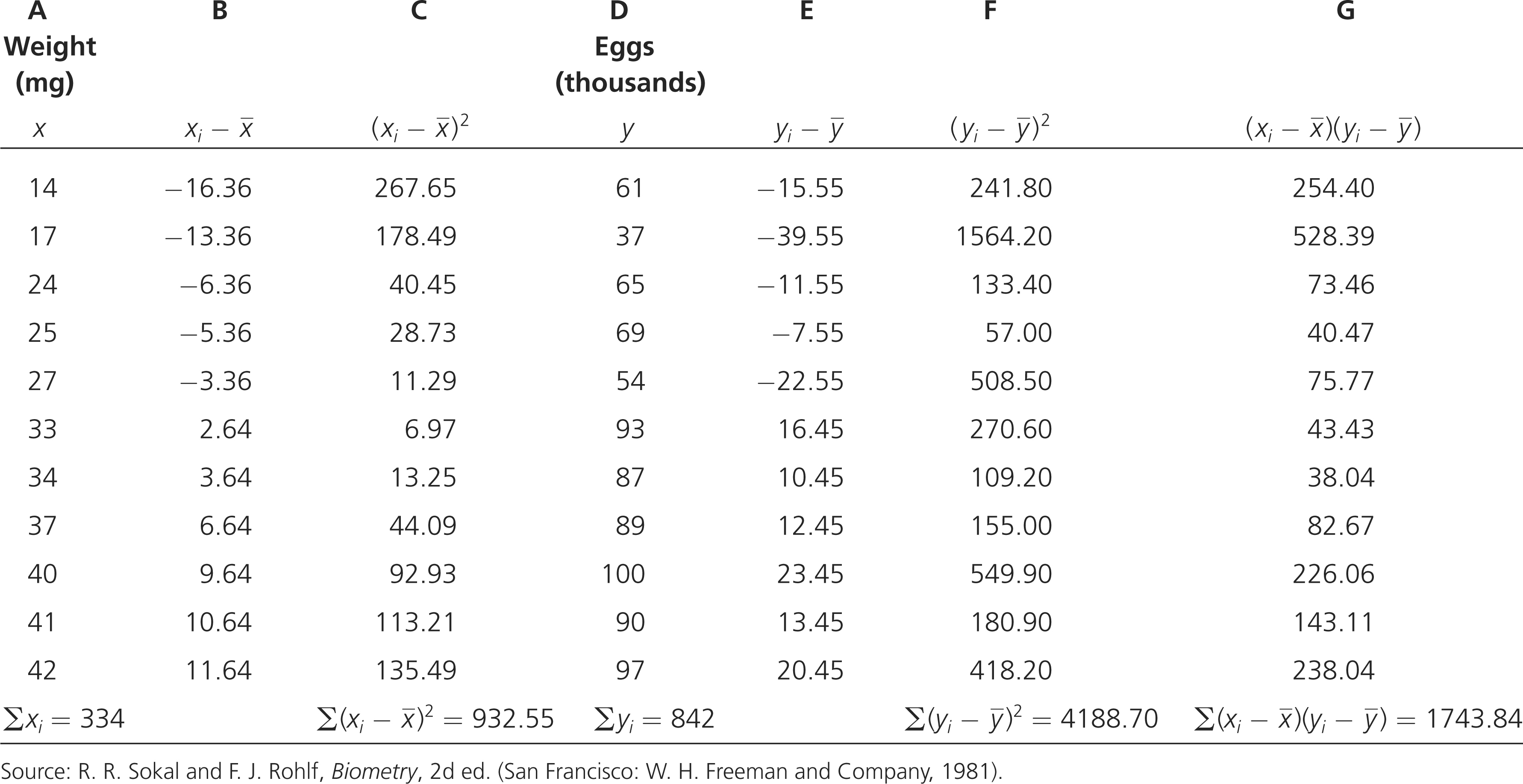
What are the correlation coefficient and the regression coefficient for body weight and egg number in these 11 fishes?
Solution Strategy
What information is required in your answer to the problem?
The correlation coefficient (r) and the regression coefficient (b) for body weight and egg number in the fish.
What information is provided to solve the problem?
Body weights and egg numbers for a sample of 11 fish.
Solution Steps
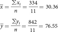
The computations needed to answer this question are given in the next table. To calculate the correlation and regression coefficients, we first obtain the sum of all the xi values (Σxi) and the sum of all the yi values (Σyi); these sums are shown in the last row of the table. We can calculate the means of the two variables by dividing the sums by the number of measurements, which is 11:
After the means have been calculated, the deviations of each value from the mean are computed; these deviations are shown in columns B and E of the table. The deviations are then squared (columns C and F) and summed (last row of columns C and F). Next, the products of the deviation of the x values and the deviation of the y values 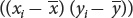 are calculated; these products are shown in column G, and their sum is shown in the last row of column G.
695
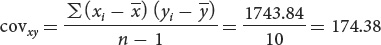
To calculate the covariance, we use Equation 24.6:
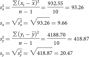
To calculate the correlation and the regression requires the variances and standard deviations of x and y:
We can now compute the correlation and regression coefficients as shown here.
Correlation coefficient:
Regression coefficient:
Practice your understanding of correlation and regression by working Problem 26 at the end of the chapter.
Applying Statistics to the Study of a Polygenic Characteristic
Edward East carried out an early statistical study of polygenic inheritance on the length of flowers in tobacco (Nicotiana longiflora). He obtained two varieties of tobacco that differed in flower length: one variety had a mean flower length of 40.5 mm, and the other had a mean flower length of 93.3 mm (Figure 24.15). These two varieties had been inbred for many generations and were homozygous at all loci contributing to flower length. Thus, there was no genetic variation in the original parental strains; the small differences in flower length within each strain were due to environmental effects on flower length.
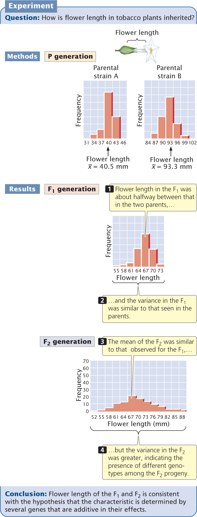
When East crossed the two strains, he found that flower length in the F1 was about halfway between that in the two parents (see Figure 24.15), as would be expected if the genes determining the differences in the two strains were additive in their effects. The variance of flower length in the F1 was similar to that seen in the parents, because all the F1 had the same genotype, as did each parental strain (the F1 were all heterozygous at the genes that differed between the two parental varieties).
696
East then interbred the F1 to produce F2 progeny. The mean flower length of the F2 was similar to that of the F1, but the variance of the F2 was much greater (see Figure 24.15). This greater variability indicates that not all of the F2 progeny had the same genotype.
East selected some F2 plants and interbred them to produce F3 progeny. He found that flower length of the F3 depended on flower length in the plants selected as their parents. This finding demonstrated that flower-length differences in the F2 were partly genetic and were therefore passed to the next generation. None of the 444 F2 plants raised by East exhibited flower lengths similar to those of the two parental strains. This result suggested that more than four loci with pairs of alleles affected flower length in his varieties, because four allelic pairs are expected to produce 1 of 256 progeny  having one or the other of the original parental phenotypes.