25.2 The Hardy–Weinberg Law Describes the Effect of Reproduction on Genotypic and Allelic Frequencies
The primary goal of population genetics is to understand the processes that shape a population’s gene pool. First, we must ask what effects reproduction and Mendelian principles have on the genotypic and allelic frequencies: How do the segregation of alleles in gamete formation and the combining of alleles in fertilization influence the gene pool? The answer to this question lies in the Hardy–Weinberg law, among the most important principles of population genetics.
The Hardy–Weinberg law was formulated independently by G. H. Hardy and Wilhelm Weinberg in 1908 (similar conclusions were reached by several other geneticists at about the same time). The law is actually a mathematical model that evaluates the effect of reproduction on the genotypic and allelic frequencies of a population. It makes several simplifying assumptions about the population and provides two key predictions if these assumptions are met. For an autosomal locus with two alleles, the Hardy–Weinberg law can be stated as follows:
Assumptions If a population is large, randomly mating, and not affected by mutation, migration, or natural selection, then:
Prediction 1 the allelic frequencies of a population do not change; and
Prediction 2 the genotypic frequencies stabilize (will not change) after one generation in the proportions p2 (the frequency of AA), 2pq (the frequency of Aa), and q2 (the frequency of aa), where p equals the frequency of allele A and q equals the frequency of allele a.
The Hardy–Weinberg law indicates that, when the assumptions are met, reproduction alone does not alter allelic or genotypic frequencies and the allelic frequencies determine the frequencies of genotypes.
The statement that genotypic frequencies stabilize after one generation means that they may change in the first generation after random mating because one generation of random mating is required to produce Hardy–Weinberg proportions of the genotypes. Afterward, the genotypic frequencies, like allelic frequencies, do not change as long as the population continues to meet the assumptions of the Hardy–Weinberg law. When genotypes are in the expected proportions of p2, 2pq, and q2, the population is said to be in Hardy–Weinberg equilibrium.
CONCEPTS
The Hardy–Weinberg law describes how reproduction and Mendelian principles affect the allelic and genotypic frequencies of a population.
 CONCEPT CHECK 2
Which statement is not an assumption of the Hardy–Weinberg law?
- The allelic frequencies (p and q) are equal.
- The population is randomly mating.
- The population is large.
- Natural selection has no effect.
Genotypic Frequencies at Hardy–Weinberg Equilibrium
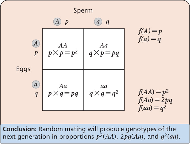
How do the conditions of the Hardy–Weinberg law lead to genotypic proportions of p2, 2pq, and q2? Mendel’s principle of segregation says that each individual organism possesses two alleles at a locus and that each of the two alleles has an equal probability of passing into a gamete. Thus, the frequencies of alleles in gametes will be the same as the frequencies of alleles in the parents. Suppose that we have a Mendelian population in which the frequencies of alleles A and a are p and q, respectively. These frequencies will also be those in the gametes. If mating is random (one of the assumptions of the Hardy–Weinberg law), the gametes will come together in random combinations, which can be represented by a Punnett square (Figure 25.2).
720
The multiplication rule of probability (Chapter 3) can be used to determine the probability of various gametes pairing. For example, the probability of a sperm containing allele A is p and the probability of an egg containing allele A is p. Applying the multiplication rule, we find that the probability that these two gametes will combine to produce an AA homozygote is p × p = p2. Similarly, the probability of a sperm containing allele a combining with an egg containing allele a to produce an aa homozygote is q × q = q2. An Aa heterozygote can be produced in one of two ways: (1) a sperm containing allele A may combine with an egg containing allele a (p × q) or (2) an egg containing allele A may combine with a sperm containing allele a (p × q). Thus, the probability of alleles A and a combining to produce an Aa heterozygote is 2pq. In summary, whenever the frequencies of alleles in a random mating population are p and q, the frequencies of the genotypes in the next generation will be p2, 2pq, and q2. Figure 25.2 demonstrates that only a single generation of random mating is required to produce the Hardy–Weinberg genotypic proportions.
Closer Examination of the Hardy–Weinberg Law
Before we consider the implications of the Hardy–Weinberg law, we need to take a closer look at the three assumptions that it makes about a population. First, it assumes that the population is large. How big is “large”? Theoretically, the Hardy–Weinberg law requires that a population be infinitely large in size, but this requirement is obviously unrealistic. In practice, many large populations are in the predicted Hardy–Weinberg proportions, and significant deviations arise only when population size is rather small. Later in the chapter, we will examine the effects of small population size on allelic frequencies.
The second assumption of the Hardy–Weinberg law is that members of the population mate randomly, which means that each genotype mates relative to its frequency. For example, suppose that three genotypes are present in a population in the following proportions: f(AA) = 0.6, f(Aa) = 0.3, and f(aa) = 0.1. With random mating, the frequency of mating between two AA homozygotes (AA × AA) will be equal to the multiplication of their frequencies: 0.6 × 0.6 = 0.36, whereas the frequency of mating between two aa homozygotes (aa × aa) will be only 0.1 × 0.1 = 0.01.
The third assumption of the Hardy–Weinberg law is that the allelic frequencies of the population are not affected by natural selection, migration, and mutation. Although mutation occurs in every population, its rate is so low that it has little short-term effect on the predictions of the Hardy–Weinberg law (although it may largely shape allelic frequencies over long periods of time when no other forces are acting). Although natural selection and migration are significant factors in real populations, we must remember that the purpose of the Hardy–Weinberg law is to examine only the effect of reproduction on the gene pool. When this effect is known, the effects of other factors (such as migration and natural selection) can be examined.
A final point is that the assumptions of the Hardy–Weinberg law apply to a single locus. No real population mates randomly for all traits, and a population is not completely free of natural selection for all traits. The Hardy–Weinberg law, however, does not require random mating and the absence of selection, migration, and mutation for all traits; it requires these conditions only for the locus under consideration. A population may be in Hardy–Weinberg equilibrium for one locus but not for others.
Implications of the Hardy–Weinberg Law
The Hardy–Weinberg law has several important implications for the genetic structure of a population. One implication is that a population cannot evolve if it meets the Hardy–Weinberg assumptions, because evolution consists of change in the allelic frequencies of a population. Therefore the Hardy–Weinberg law tells us that reproduction alone will not bring about evolution. Other processes such as natural selection, mutation, migration, or chance are required for populations to evolve.
A second important implication is that, when a population is in Hardy–Weinberg equilibrium, the genotypic frequencies are determined by the allelic frequencies. When a population is not in Hardy–Weinberg equilibrium, we have no basis for predicting the genotypic frequencies. Although we can always determine the allelic frequencies from the genotypic frequencies (see Equation 25.3), the reverse (determining the genotypic frequencies from the allelic frequencies) is possible only when the population is in Hardy–Weinberg equilibrium.
721
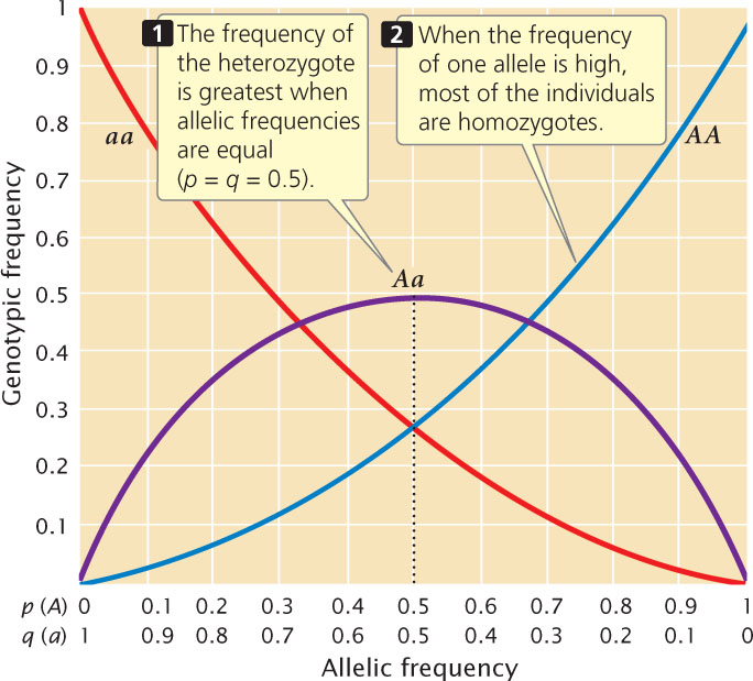
For a locus with two alleles, the frequency of the heterozygote is greatest when allelic frequencies are between 0.33 and 0.66 and is at a maximum when allelic frequencies are each 0.5 (Figure 25.3). The heterozygote frequency also never exceeds 0.5 when the population is in Hardy–Weinberg equilibrium. Furthermore, when the frequency of one allele is low, homozygotes for that allele will be rare, and most of the copies of a rare allele will be present in heterozygotes. As you can see from Figure 25.3, when the frequency of allele a is 0.2, the frequency of the aa homozygote is only 0.04 (q2), but the frequency of Aa heterozygotes is 0.32 (2pq); 80% of the a alleles are in heterozygotes.  Use Animation 25.1 to examine the effect of allelic frequencies on genotypic frequencies when a population is in Hardy–Weinberg equilibrium.
A third implication of the Hardy–Weinberg law is that a single generation of random mating produces the equilibrium frequencies of p2, 2pq, and q2. The fact that genotypes are in Hardy–Weinberg proportions does not prove that the population is free from natural selection, mutation, and migration. It means only that these forces have not acted since the last time random mating took place.
Extensions of the Hardy–Weinberg Law
The Hardy–Weinberg expected proportions can also be applied to multiple alleles and X-linked alleles (Table 25.1). With multiple alleles, the genotypic frequencies expected at equilibrium are the square of the allelic frequencies. For an autosomal locus with three alleles, the equilibrium genotypic frequencies will (p + q + r)2 = p2 + 2pq + q2 + 2pr + 2qr + r2. For an X-linked locus with two alleles, XA and Xa, the equilibrium frequencies of the female genotypes are (p + q)2 = p2 + 2pq + q2, where p2 is the frequency of XAXA, 2pq is the frequency of XAXa, and q2 is the frequency of XaXa. Males have only a single X-linked allele, and so the frequencies of the male genotypes are p (frequency of XAY) and q (frequency of XaY). These proportions are those of the genotypes among males and females rather than the proportions among the entire population. Thus, p2 is the expected proportion of females with the genotype XAXA; if females make up 50% of the population, then the expected proportion of this genotype in the entire population is 0.5 × p2.
| Situation | Allelic Frequencies | Genotypic Frequencies |
|---|---|---|
| Three alleles | f(A1) = p | f(A1A1) = p2 |
| f(A2) = q | f(A1A2) = 2pq | |
| f(A3) = r | f(A2A2) = q2 | |
| f(A1A3) = 2pr | ||
| f(A2A3) = 2qr | ||
| f(A3A3) = r2 | ||
| X-linked alleles | f(x1) = p | f(X1X1 female) = p2 |
| f(X2) = q | f(X1X2 female) = 2pq | |
| f(X2X2 female) = q2 | ||
| f(X1Y male) = p | ||
| f(X2Y male) = q | ||
| Note: For X-linked female genotypes, the frequencies are the proportions among all females; for X-linked male genotypes, the frequencies are the proportions among all males. | ||
The frequency of an X-linked recessive trait among males is q, whereas the frequency among females is q2. When an X-linked allele is uncommon, the trait will therefore be much more frequent in males than in females. Consider hemophilia A, a clotting disorder caused by an X-linked recessive allele with a frequency (q) of approximately 1 in 10,000, or 0.0001. At Hardy–Weinberg equilibrium, this frequency will also be the frequency of the disease among males. The frequency of the disease among females, however, will be q2 = (0.0001)2 = 0.00000001, which is only 1 in 100 million. Hemophilia is 10,000 times as frequent in males as in females.
Testing for Hardy–Weinberg Proportions
To determine if a population’s genotypes are in Hardy–Weinberg equilibrium, the genotypic proportions expected under the Hardy–Weinberg law must be compared with the observed genotypic frequencies. To do so, we first calculate the allelic frequencies, then find the expected genotypic frequencies by using the square of the allelic frequencies, and, finally, compare the observed and expected genotypic frequencies by using a chi-square test.
722
WORKED PROBLEM
Jeffrey Mitton and his colleagues found three genotypes (R2R2, R2R3, and R3R3) at a locus encoding the enzyme peroxidase in ponderosa pine trees growing at Glacier Lake, Colorado. The observed numbers of these genotypes were:
| Genotypes | Number observed |
|---|---|
| R2R2 | 135 |
| R2R3 | 44 |
| R3R3 | 11 |
Are the ponderosa pine trees at Glacier Lake in Hardy–Weinberg equilibrium at the peroxidase locus?
Solution Strategy
What information is required in your answer to the problem?
The results of a chi-square test to determine whether the population is in Hardy–Weinberg equilibrium.
What information is provided to solve the problem?
The numbers of the different genotypes in a sample of the population.
Solution Steps
If the frequency of the R2 allele equals p and the frequency of the R3 allele equals q, the frequency of the R2 allele is:
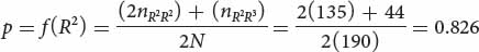
The frequency of the R3 allele is obtained by subtraction:
q = f(R3) = 1 − p = 0.174
The frequencies of the genotypes expected under Hardy–Weinberg equilibrium are then calculated by using p2, 2pq, and q2:
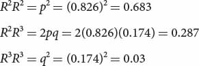
Multiplying each of these expected genotypic frequencies by the total number of observed genotypes in the sample (190), we obtain the numbers expected for each genotype:
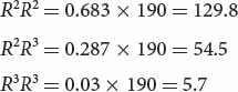
By comparing these expected numbers with the observed numbers of each genotype, we see that there are more R2R2 and R3R3 homozygotes and fewer R2R3 heterozygotes in the population than we expect at equilibrium.
A chi-square goodness-of-fit test is used to determine whether the differences between the observed and the expected numbers of each genotype are due to chance:
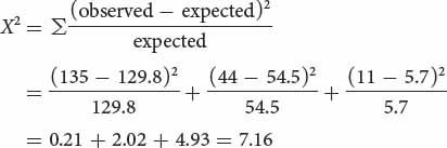
The calculated chi-square value is 7.16; to obtain the probability associated with this chi-square value, we determine the appropriate degrees of freedom.
Up to this point, the chi-square test for assessing Hardy–Weinberg equilibrium has been identical with the chi-square tests that we used in Chapter 3 to assess progeny ratios in a genetic cross, where the degrees of freedom were n − 1 and n equaled the number of expected genotypes. For the Hardy–Weinberg test, however, we must subtract an additional degree of freedom, because the expected numbers are based on the observed allelic frequencies; therefore, the observed numbers are not completely free to vary. In general, the degrees of freedom for a chi-square test of Hardy–Weinberg equilibrium equal the number of expected genotypic classes minus the number of associated alleles. For this particular Hardy–Weinberg test, the degree of freedom is 3 − 2 = 1.
After we have calculated both the chi-square value and the degrees of freedom, the probability associated with this value can be sought in a chi-square table (see Table 3.7). With one degree of freedom, a chi-square value of 7.16 has a probability between 0.01 and 0.001. It is very unlikely that the peroxidase genotypes observed at Glacier Lake are in Hardy–Weinberg proportions.
For additional practice, determine whether the genotypic frequencies in Problem 22 at the end of the chapter are in Hardy–Weinberg equilibrium.
CONCEPTS
The observed number of genotypes in a population can be compared with the Hardy–Weinberg expected proportions by using a chi-square goodness-of-fit test.
CONCEPT CHECK 3
What is the expected frequency of heterozygotes in a population with allelic frequencies x and y that is in Hardy–Weinberg equilibrium?
- x + y
- xy
- 2xy
- (x − y)2
Estimating Allelic Frequencies with the Hardy–Weinberg Law
A practical use of the Hardy–Weinberg law is that it allows us to calculate allelic frequencies when dominance is present. For example, cystic fibrosis is an autosomal recessive disorder characterized by respiratory infections, incomplete digestion, and abnormal sweating. Among North American Caucasians, the incidence of the disease is approximately 1 person in 2000. The formula for calculating allelic frequency (see Equation 25.3) requires that we know the numbers of homozygotes and heterozygotes, but cystic fibrosis is a recessive disease and so we cannot easily distinguish between homozygous unaffected persons and heterozygous carriers. Although molecular tests are available for identifying heterozygous carriers of the cystic fibrosis gene, the low frequency of the disease makes widespread screening impractical. In such situations, the Hardy–Weinberg law can be used to estimate the allelic frequencies.
723
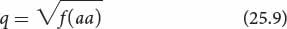
If we assume that a population is in Hardy–Weinberg equilibrium with regard to this locus, then the frequency of the recessive genotype (aa) will be q2, and the allelic frequency is the square root of the genotypic frequency:
If the frequency of cystic fibrosis in North American Caucasians is approximately 1 in 2000, or 0.0005, then 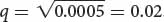 . Thus, about 2% of the alleles in the Caucasian population encode cystic fibrosis. We can calculate the frequency of the normal allele by subtracting: p = 1 − q = 1 − 0.02 = 0.98. After we have calculated p and q, we can use the Hardy–Weinberg law to determine the frequencies of homozygous unaffected people and heterozygous carriers of the gene:
Thus, about 4% (1 of 25) of Caucasians are heterozygous carriers of the allele that causes cystic fibrosis. ![]() TRY PROBLEM 25
TRY PROBLEM 25
CONCEPTS
Although allelic frequencies cannot be calculated directly for traits that exhibit dominance, the Hardy–Weinberg law can be used to estimate the allelic frequencies if the population is in Hardy-Weinberg equilibrium for that locus. The frequency of the recessive allele will be equal to the square root of the frequency of the recessive trait.
CONCEPT CHECK 4
In cats, all-white color is dominant over not all-white. In a population of 100 cats, 19 are all-white. Assuming that the population is in Hardy–Weinberg equilibrium, what is the frequency of the all-white allele in this population?