3.2 Monohybrid Crosses Reveal the Principle of Segregation and the Concept of Dominance
Mendel started with 34 varieties of peas and spent 2 years selecting those varieties that he would use in his experiments. He verified that each variety was pure-breeding (homozygous for each of the traits that he chose to study) by growing the plants for two generations and confirming that all offspring were the same as their parents. He then carried out a number of crosses between the different varieties. Although peas are normally self-fertilizing (each plant crosses with itself), Mendel conducted crosses between different plants by opening the buds before the anthers (male sex organs) were fully developed, removing the anthers, and then dusting the stigma (female sex organs) with pollen from a different plant’s anthers (Figure 3.4).
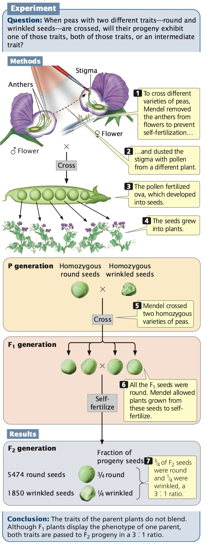
Mendel began by studying monohybrid crosses—those between parents that differed in a single characteristic. In one experiment, Mendel crossed a pure-breeding (homozygous) pea plant for round seeds with one that was pure-breeding for wrinkled seeds (see Figure 3.4). This first generation of a cross is the P (parental) generation.
50
After crossing the two varieties in the P generation, Mendel observed the offspring that resulted from the cross. In regard to seed characteristics, such as seed shape, the phenotype develops as soon as the seed matures because the seed traits are determined by the newly formed embryo within the seed. For characteristics associated with the plant itself, such as stem length, the phenotype doesn’t develop until the plant grows from the seed; for these characteristics, Mendel had to wait until the following spring, plant the seeds, and then observe the phenotypes on the plants that germinated.
The offspring from the parents in the P generation are the F1 (first filial) generation. When Mendel examined the F1 generation of this cross, he found that they expressed only one of the phenotypes present in the parental generation: all the F1 seeds were round. Mendel carried out 60 such crosses and always obtained this result. He also conducted reciprocal crosses: in one cross, pollen (the male gamete) was taken from a plant with round seeds and, in its reciprocal cross, pollen was taken from a plant with wrinkled seeds. Reciprocal crosses gave the same result: all the F1 were round.
Mendel wasn’t content with examining only the seeds arising from these monohybrid crosses. The following spring, he planted the F1 seeds, cultivated the plants that germinated from them, and allowed the plants to self fertilize, producing a second generation—the F2 (second filial) generation. Both of the traits from the P generation emerged in the F2 generation; Mendel counted 5474 round seeds and 1850 wrinkled seeds in the F2 (see Figure 3.4). He noticed that the number of the round and wrinkled seeds constituted approximately a 3 to 1 ratio; that is, about  of the F2 seeds were round and
  were wrinkled. Mendel conducted monohybrid crosses for all seven of the characteristics that he studied in pea plants and, in all of the crosses, he obtained the same result: all of the F1 resembled only one of the two parents, but both parental traits emerged in the F2 in an approximate ratio of 3 : 1.
What Monohybrid Crosses Reveal
First, Mendel reasoned that, although the F1 plants display the phenotype of only one parent, they must inherit genetic factors from both parents because they transmit both phenotypes to the F2 generation. The presence of both round and wrinkled seeds in the F2 plants could be explained only if the F1 plants possessed both round and wrinkled genetic factors that they had inherited from the P generation. He concluded that each plant must therefore possess two genetic factors encoding a characteristic.
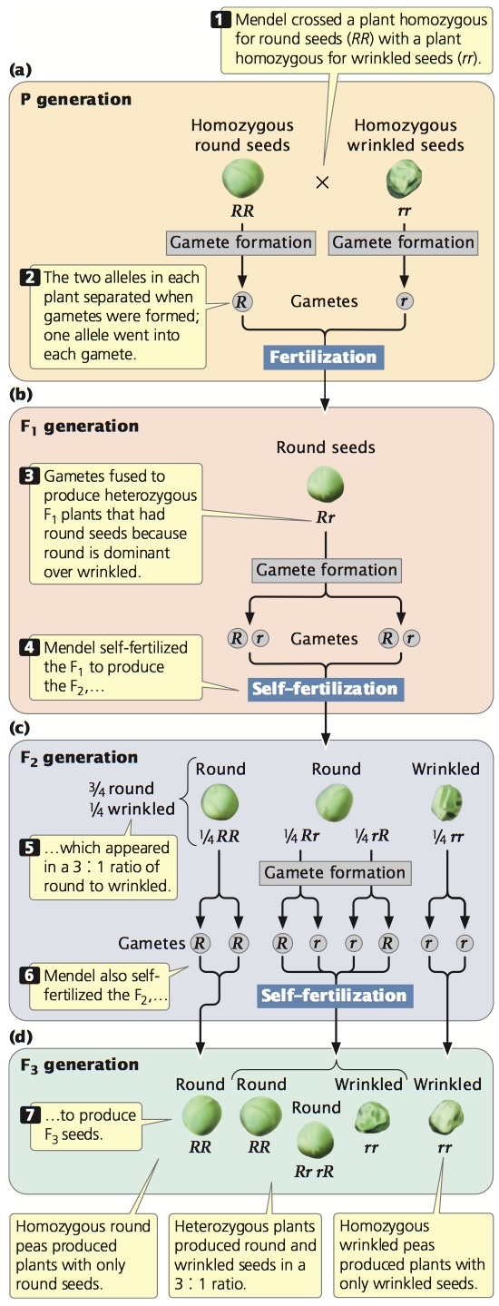
The genetic factors (now called alleles) that Mendel discovered are, by convention, designated with letters; the allele for round seeds is usually represented by R, and the allele for wrinkled seeds by r. The plants in the P generation of Mendel’s cross possessed two identical alleles: RR in the round-seeded parent and rr in the wrinkled-seeded parent (Figure 3.5a).
51
The second conclusion that Mendel drew from his monohybrid crosses was that the two alleles in each plant separate when gametes are formed, and one allele goes into each gamete. When two gametes (one from each parent) fuse to produce a zygote, the allele from the male parent unites with the allele from the female parent to produce the genotype of the offspring. Thus, Mendel’s F1 plants inherited an R allele from the round-seeded plant and an r allele from the wrinkled-seeded plant (Figure 3.5b). However, only the trait encoded by the round allele (R) was observed in the F1: all the F1 progeny had round seeds. Those traits that appeared unchanged in the F1 heterozygous offspring Mendel called dominant, and those traits that disappeared in the F1 heterozygous offspring he called recessive. Alleles for dominant traits are often symbolized with uppercase letters (e.g. R), while alleles for recessive traits are often symbolized with lowercase letters (e.g. r). When dominant and recessive alleles are present together, the recessive allele is masked, or suppressed. The concept of dominance was the third important conclusion that Mendel derived from his monohybrid crosses.
Mendel’s fourth conclusion was that the two alleles of an individual plant separate with equal probability into the gametes. When plants of the F1 (with genotype Rr) produced gametes, half of the gametes received the R allele for round seeds and half received the r allele for wrinkled seeds. The gametes then paired randomly to produce the following genotypes in equal proportions among the F2: RR, Rr, rR, rr (Figure 3.5c). Because round (R) is dominant over wrinkled (r), there were three round progeny in the F2 (RR, Rr, rR) for every one wrinkled progeny (rr) in the F2. This 3 : 1 ratio of round to wrinkled progeny that Mendel observed in the F2 could be obtained only if the two alleles of a genotype separated into the gametes with equal probability.
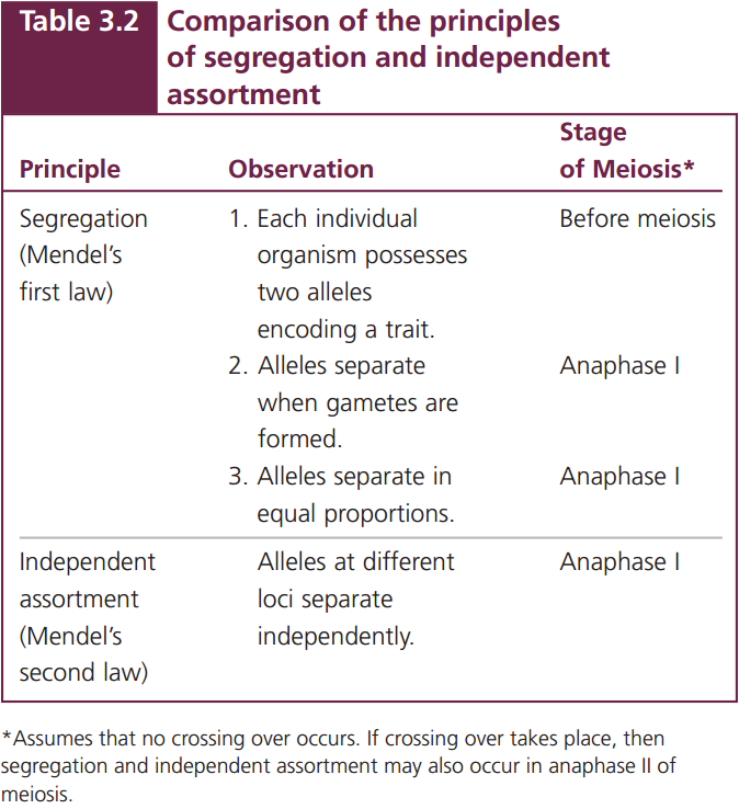
The conclusions that Mendel developed about inheritance from his monohybrid crosses have been further developed and formalized into the principle of segregation and the concept of dominance. The principle of segregation (Mendel’s first law, see Table 3.2) states that each individual diploid organism possesses two alleles for any particular characteristic, one inherited from the maternal parent and one from the paternal parent. These two alleles segregate (separate) when gametes are formed, and one allele goes into each gamete. Furthermore, the two alleles segregate into gametes in equal proportions. The concept of dominance states that, when two different alleles are present in a genotype, only the trait encoded by one of them—the “dominant” allele—is observed in the phenotype.
Mendel confirmed these principles by allowing his F2 plants to self-fertilize and produce an F3 generation. He found that the plants grown from the wrinkled seeds—those displaying the recessive trait (rr)—produced an F3 in which all plants produced wrinkled seeds. Because his wrinkled-seeded plants were homozygous for wrinkled alleles (rr), only wrinkled alleles could be passed on to their progeny (Figure 3.5d).
The plants grown from round seeds—the dominant trait—fell into two types (see Figure 3.5c). On self-fertilization, about  of these plants produced both round and wrinkled seeds in the F3 generation. These plants were heterozygous (Rr); so they produced
RR (round),
of these plants produced both round and wrinkled seeds in the F3 generation. These plants were heterozygous (Rr); so they produced
RR (round),  Rr (round), and
rr (wrinkled) seeds, giving a 3 : 1 ratio of round to wrinkled in the F3. About
Rr (round), and
rr (wrinkled) seeds, giving a 3 : 1 ratio of round to wrinkled in the F3. About  of the plants grown from round seeds were of the second type; they produced only the round-seeded trait in the F3. These plants were homozygous for the round allele (RR) and could thus produce only round offspring in the F3 generation. Mendel planted the seeds obtained in the F3 and carried these plants through three more rounds of self-fertilization. In each generation,
of the round-seeded plants produced round and wrinkled offspring, whereas
produced only round offspring. These results are entirely consistent with the principle of segregation.
of the plants grown from round seeds were of the second type; they produced only the round-seeded trait in the F3. These plants were homozygous for the round allele (RR) and could thus produce only round offspring in the F3 generation. Mendel planted the seeds obtained in the F3 and carried these plants through three more rounds of self-fertilization. In each generation,
of the round-seeded plants produced round and wrinkled offspring, whereas
produced only round offspring. These results are entirely consistent with the principle of segregation.
CONCEPTS
The principle of segregation states that each individual organism possesses two alleles that can encode a characteristic. These alleles segregate when gametes are formed, and one allele goes into each gamete. The concept of dominance states that, when the two alleles of a genotype are different, only the trait encoded by one of them—the “dominant” allele—is observed.
 CONCEPT CHECK 3
How did Mendel know that each of his pea plants carried two alleles encoding a characteristic?
52
CONNECTING CONCEPTS: Relating Genetic Crosses to Meiosis
We have now seen how the results of monohybrid crosses are explained by Mendel’s principle of segregation. Many students find that they enjoy working genetic crosses but are frustrated by the abstract nature of the symbols. Perhaps you feel the same at this point. You may be asking, “What do these symbols really represent? What does the genotype RR mean in regard to the biology of the organism?” The answers to these questions lie in relating the abstract symbols of crosses to the structure and behavior of chromosomes, the repositories of genetic information (see Chapter 2).
In 1900, when Mendel’s work was rediscovered and biologists began to apply his principles of heredity, the relation between genes and chromosomes was still unclear. The theory that genes are located on chromosomes (the chromosome theory of heredity) was developed in the early 1900s by Walter Sutton, then a graduate student at Columbia University. Through the careful study of meiosis in insects, Sutton documented the fact that each homologous pair of chromosomes consists of one maternal chromosome and one paternal chromosome. Showing that these pairs segregate independently into gametes in meiosis, he concluded that this process is the biological basis for Mendel’s principles of heredity. German cytologist and embryologist Theodor Boveri came to similar conclusions at about the same time.
53
The symbols used in genetic crosses, such as R and r, are just shorthand notations for particular sequences of DNA in the chromosomes that encode particular phenotypes. The two alleles of a genotype are found on different but homologous chromosomes. One chromosome of each homologous pair is inherited from the mother and the other is inherited from the father. In the S phase of meiotic interphase, each chromosome replicates, producing two copies of each allele, one on each chromatid (Figure 3.6a). The homologous chromosomes segregate in anaphase I, thereby separating the two different alleles (Figure 3.6b and c). This chromosome segregation is the basis of the principle of segregation. In anaphase II of meiosis, the two chromatids of each replicated chromosome separate; so each gamete resulting from meiosis carries only a single allele at each locus, as Mendel’s principle of segregation predicts.
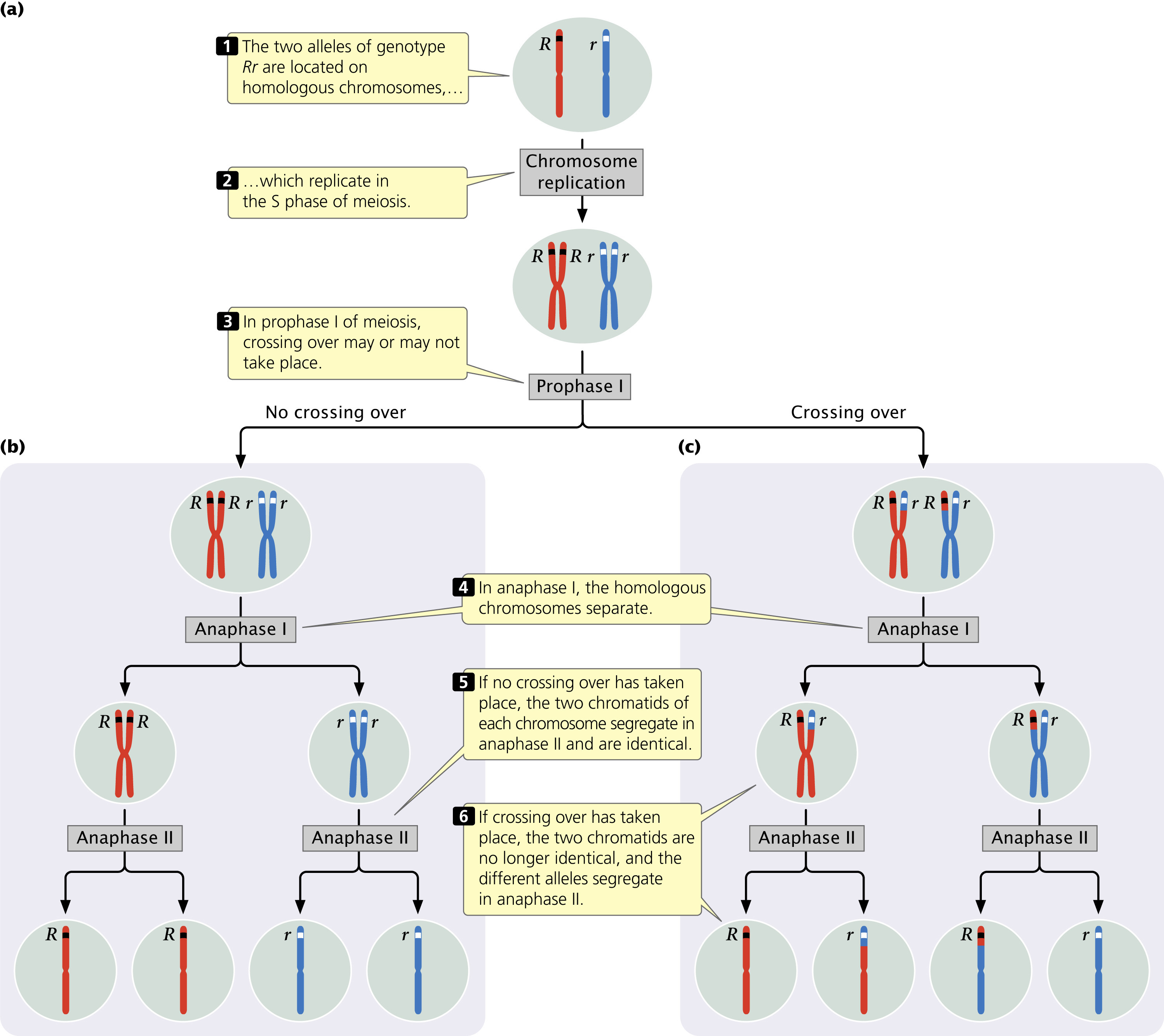
If crossing over has taken place in prophase I of meiosis, then the two chromatids of each replicated chromosome are no longer identical, and the segregation of different alleles takes place at anaphase I and anaphase II (see Figure 3.6c). However, Mendel didn’t know anything about chromosomes; he formulated his principles of heredity entirely on the basis of the results of the crosses that he carried out. Nevertheless, we should not forget that these principles work because they are based on the behavior of actual chromosomes in meiosis. ![]() TRY PROBLEM 30
TRY PROBLEM 30
The Molecular Nature of Alleles
Let’s take a moment to consider in more detail exactly what an allele is and how it determines a phenotype. Although Mendel had no information about the physical nature of the genetic factors in his crosses, modern geneticists have now determined the molecular basis of these factors and how they encode a trait like wrinkled peas.
Alleles, such as R and r that code for round and wrinkled peas, usually represent specific DNA sequences. The locus that determines whether a pea is round or wrinkled is a sequence of DNA on pea chromosome 5 that encodes a protein called starch-branching enzyme isoform 1 (SBEI). The R allele, which produces round seeds in pea plants, codes for a normal, functional form of the SBEI enzyme. This enzyme converts a linear form of starch into a highly branched form. The r allele, which encodes wrinkled seeds, is a different DNA sequence that contains a mutation or error; it encodes a nonactive form of the enzyme that does not produce the branched form of starch and leads to the accumulation of sucrose within the rr pea. Because the rr pea contains a large amount of sucrose, the developing seed absorbs water and swells. Later, as the pea matures, it loses water. Because rr peas absorbed more water and expanded more during development, they lose more water during maturation and afterwards appear shriveled or wrinkled. The r allele for wrinkled seeds is recessive because the presence of a single R allele in the heterozygote encodes enough SBEI enzyme to produce branched starch and round seeds.
Research has revealed that the r allele contains an extra 800 base pairs of DNA that disrupt the normal coding sequence of the gene. The extra DNA appears to have come from a transposable element, a type of DNA sequence that has the ability to move from one location in the genome to another, which we will discuss further in Chapter 18.
Predicting the Outcomes of Genetic Crosses
One of Mendel’s goals in conducting his experiments on pea plants was to develop a way to predict the outcome of crosses between plants with different phenotypes. In this section, you will first learn a simple, shorthand method for predicting outcomes of genetic crosses (the Punnett square), and then you will learn how to use probability to predict the results of crosses.
The Punnett Square"The Punnett square was developed by English geneticist Reginald C. Punnett in 1917. To illustrate the Punnett square, let’s examine another cross carried out by Mendel. By crossing two varieties of peas that differed in height, Mendel established that tall (T) was dominant over short (t). He tested his theory concerning the inheritance of dominant traits by crossing an F1 tall plant that was heterozygous (Tt) with the short homozygous parental variety (tt). This type of cross, between an F1 genotype and either of the parental genotypes, is called a backcross.
To predict the types of offspring that result from this backcross, we first determine which gametes will be produced by each parent (Figure 3.7a). The principle of segregation tells us that the two alleles in each parent separate, and one allele passes to each gamete. All gametes from the homozygous tt short plant will receive a single short (t) allele. The tall plant in this cross is heterozygous (Tt); so 50% of its gametes will receive a tall allele (T) and the other 50% will receive a short allele (t).
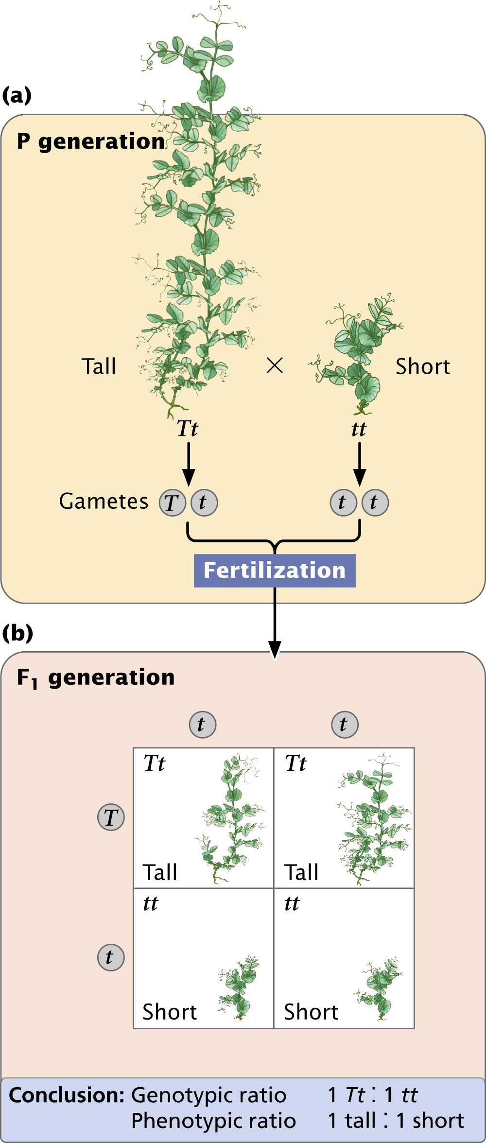
A Punnett square is constructed by drawing a grid, putting the gametes produced by one parent along the upper edge and the gametes produced by the other parent down the left side (Figure 3.7b). Each cell (a block within the Punnett square) contains an allele from each of the corresponding gametes, generating the genotype of the progeny produced by fusion of those gametes. In the upper left-hand cell of the Punnett square in Figure 3.7b, a gamete containing T from the tall plant unites with a gamete containing t from the short plant, giving the genotype of the progeny (Tt). It is useful to write the phenotype expressed by each genotype; here the progeny will be tall, because the tall allele is dominant over the short allele. This process is repeated for all the cells in the Punnett square.
By simply counting, we can determine the types of progeny produced and their ratios. In Figure 3.7b, two cells contain tall (Tt) progeny and two cells contain short (tt) progeny; so the genotypic ratio expected for this cross is 2 Tt to 2 tt (a 1 : 1 ratio). Another way to express this result is to say that we expect
of the progeny to have genotype Tt (and phenotype tall) and
of the progeny to have genotype tt (and phenotype short). In this cross, the genotypic ratio and the phenotypic ratio are the same, but this outcome need not be the case. Try completing a Punnett square for the cross in which the F1 round-seeded plants in Figure 3.5 undergo self-fertilization (you should obtain a phenotypic ratio of 3 round to 1 wrinkled and a genotypic ratio of 1 RR to 2 Rr to 1 rr).
54
CONCEPTS
The Punnett square is a shorthand method of predicting the genotypic and phenotypic ratios of progeny from a genetic cross.
CONCEPT CHECK 4
If an F1 plant depicted in Figure 3.5 is backcrossed to the parent with round seeds, what proportion of the progeny will have wrinkled seeds? (Use a Punnett square.)
-
-
-
- 0
Probability as a Tool of GeneticsAnother method for determining the outcome of a genetic cross is to use the rules of probability, as Mendel did with his crosses. Probability expresses the likelihood of the occurrence of a particular event. It is the number of times that a particular event takes place, divided by the number of all possible outcomes. For example, a deck of 52 cards contains only one king of hearts. The probability of drawing one card from the deck at random and obtaining the king of hearts is  because there is only one card that is the king of hearts (one event) and there are 52 cards that can be drawn from the deck (52 possible outcomes). The probability of drawing a card and obtaining an ace is
  because there are four cards that are aces (four events) and 52 cards (possible outcomes). Probability can be expressed either as a fraction (
in this case) or as a decimal number (0.077 in this case).
because there are four cards that are aces (four events) and 52 cards (possible outcomes). Probability can be expressed either as a fraction (
in this case) or as a decimal number (0.077 in this case).
The probability of a particular event may be determined by knowing something about how or how often the event takes place. We know, for example, that the probability of rolling a six-sided die and getting a four is  because the die has six sides and any one side is equally likely to end up on top. So, in this case, understanding the nature of the event—the shape of the thrown die—allows us to determine the probability. In other cases, we determine the probability of an event by making a large number of observations. When a weather forecaster says that there is a 40% chance of rain on a particular day, this probability was obtained by observing a large number of days with similar atmospheric conditions and finding that it rains on 40% of those days. In this case, the probability has been determined empirically (by observation).
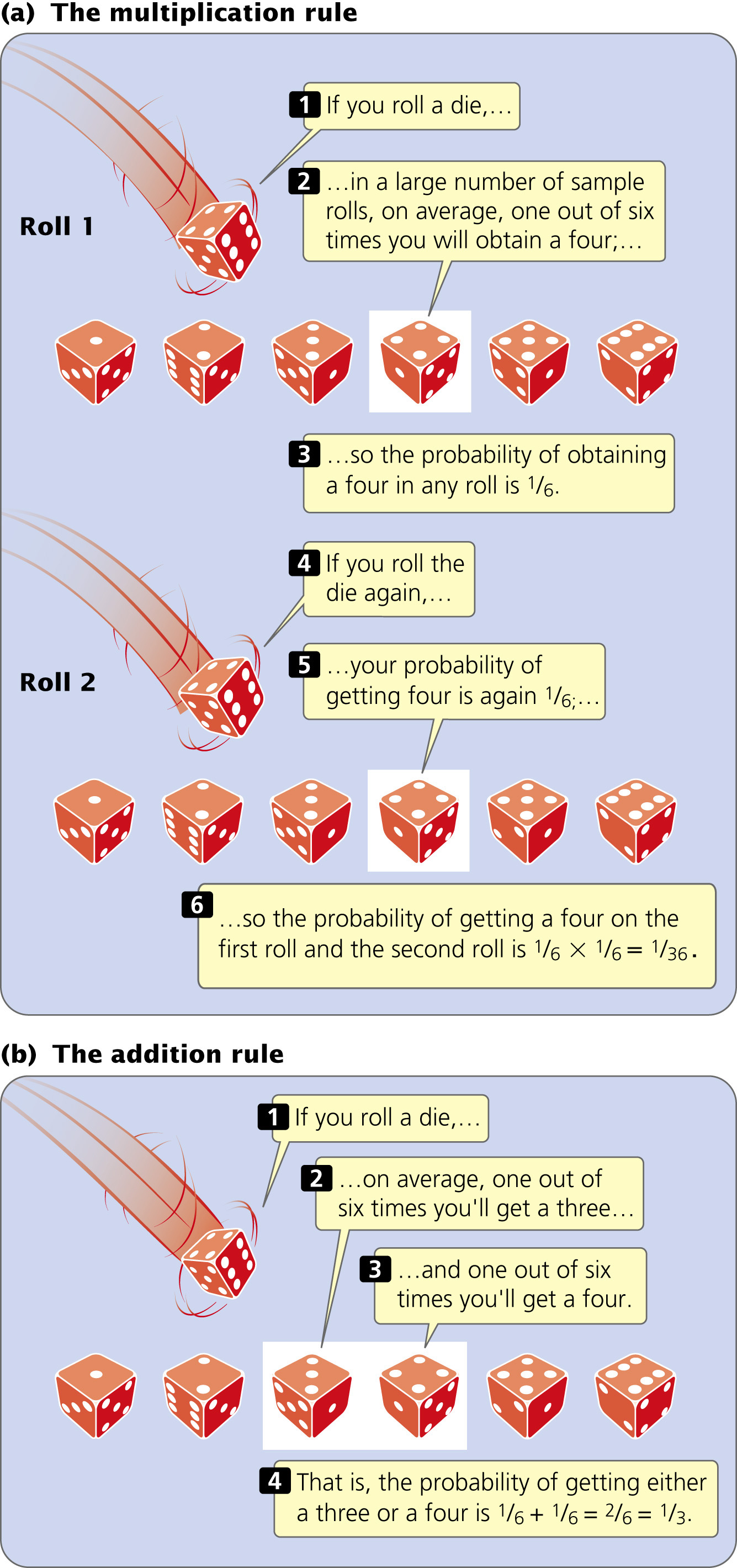
The Multiplication RuleTwo rules of probability are useful for predicting the ratios of offspring produced in genetic crosses. The first is the multiplication rule, which states that the probability of two or more independent events taking place together is calculated by multiplying their independent probabilities.
To illustrate the use of the multiplication rule, let’s again consider the roll of a die. The probability of rolling one die and obtaining a four is
. To calculate the probability of rolling a die twice and obtaining 2 fours, we can apply the multiplication rule. The probability of obtaining a four on the first roll is
and the probability of obtaining a four on the second roll is
; so the probability of rolling a four on both is
×
=  (Figure 3.8a). The key indicator for applying the multiplication rule is the word and; in the example just considered, we wanted to know the probability of obtaining a four on the first roll and a four on the second roll.
For the multiplication rule to be valid, the events whose joint probability is being calculated must be independent—the outcome of one event must not influence the outcome of the other. For example, the number that comes up on one roll of the die has no influence on the number that comes up on the other roll; so these events are independent. However, if we wanted to know the probability of being hit on the head with a hammer and going to the hospital on the same day, we could not simply apply the multiplication rule and multiply the two events together, because they are not independent—being hit on the head with a hammer certainly influences the probability of going to the hospital.
55
The Addition RuleThe second rule of probability frequently used in genetics is the addition rule, which states that the probability of any one of two or more mutually exclusive events is calculated by adding the probabilities of these events. Let’s look at this rule in concrete terms. To obtain the probability of throwing a die once and rolling either a three or a four, we would use the addition rule, adding the probability of obtaining a three (
) to the probability of obtaining a four (again,
), or
+
=  =
(Figure 3.8b). The key indicators for applying the addition rule are the words either and or.
=
(Figure 3.8b). The key indicators for applying the addition rule are the words either and or.
For the addition rule to be valid, the events whose probability is being calculated must be mutually exclusive, meaning that one event excludes the possibility of the occurrence of the other event. For example, you cannot throw a single die just once and obtain both a three and a four, because only one side of the die can be on top. These events are mutually exclusive.
CONCEPTS
The multiplication rule states that the probability of two or more independent events taking place together is calculated by multiplying their independent probabilities. The addition rule states that the probability that any one of two or more mutually exclusive events taking place is calculated by adding their probabilities.
CONCEPT CHECK 5
If the probability of being blood-type A is  and the probability of blood-type O is
, what is the probability of being either blood-type A or blood-type O?
and the probability of blood-type O is
, what is the probability of being either blood-type A or blood-type O?


Applying Probability to Genetic CrossesThe multiplication and addition rules of probability can be used in place of the Punnett square to predict the ratios of progeny expected from a genetic cross. Let’s first consider a cross between two pea plants heterozygous for the locus that determines height, Tt × Tt. Half of the gametes produced by each plant have a T allele, and the other half have a t allele; so the probability for each type of gamete is
.
The gametes from the two parents can combine in four different ways to produce offspring. Using the multiplication rule, we can determine the probability of each possible type. To calculate the probability of obtaining TT progeny, for example, we multiply the probability of receiving a T allele from the first parent (
) times the probability of receiving a T allele from the second parent (
). The multiplication rule should be used here because we need the probability of receiving a T allele from the first parent and a T allele from the second parent—two independent events. The four types of progeny from this cross and their associated probabilities are:
| TT | (T gamete and T gamete) |
×
=
|
tall |
| Tt | (T gamete and t gamete) |
×
=
|
tall |
| tT | (t gamete and T gamete) |
×
=
|
tall |
| tt | (t gamete and t gamete) |
×
=
|
short |
56
Notice that there are two ways for heterozygous progeny to be produced: a heterozygote can either receive a T allele from the first parent and a t allele from the second or receive a t allele from the first parent and a T allele from the second.
After determining the probabilities of obtaining each type of progeny, we can use the addition rule to determine the overall phenotypic ratios. Because of dominance, a tall plant can have genotype TT, Tt, or tT; so, using the addition rule, we find the probability of tall progeny to be
+
+
=
. Because only one genotype encodes short (tt), the probability of short progeny is simply
.
Two methods have now been introduced to solve genetic crosses: the Punnett square and the probability method. At this point, you may be asking, “Why bother with probability rules and calculations? The Punnett square is easier to understand and just as quick.” This is true for simple monohybrid crosses. However, for tackling more-complex crosses concerning genes at two or more loci, the probability method is both clearer and quicker than the Punnett square.
Conditional ProbabilityThus far, we have used probability to predict the chances of producing certain types of progeny given only the genotypes of the parents. Sometimes we have additional information that modifies or “conditions” the probability, a situation termed conditional probability. For example, assume that we cross two heterozygous pea plants (Tt × Tt) and obtain a tall progeny. What is the probability that this tall plant is heterozygous (Tt)? You might assume that the probability would be
, the probability of obtaining a heterozygous progeny in a cross between two heterozygotes. However, in this case we have some additional information—the phenotype of the progeny plant—which modifies the probability. When two heterozygous individuals are crossed, we expect
TT,
Tt, and
tt progeny. We know that the progeny in question is tall, so we can eliminate the possibility that it has genotype tt. Tall progeny must be either genotype TT or genotype Tt and, in a cross between two heterozygotes, these occur in a 1 : 2 ratio. Therefore, the probability that a tall progeny is heterozygous (Tt) is two out of three, or
.
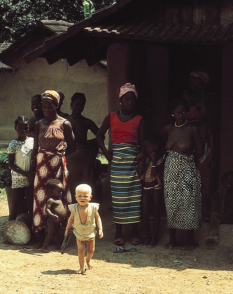
The Binomial Expansion and ProbabilityWhen probability is used, it is important to recognize that there may be several different ways in which a set of events can occur. Consider two parents who are both heterozygous for albinism, a recessive condition in humans that causes reduced pigmentation in the skin, hair, and eyes (Figure 3.9; see also the introduction to Chapter 1). When two parents heterozygous for albinism mate (Aa × Aa), the probability of their having a child with albinism (aa) is
and the probability of having a child with normal pigmentation (AA or Aa) is
. Suppose we want to know the probability of this couple having three children with albinism. In this case, there is only one way in which this can happen: their first child has albinism and their second child has albinism and their third child has albinism. Here, we simply apply the multiplication rule:
×
×
=  .
.
Suppose we now ask what the probability is of this couple having three children, one with albinism and two with normal pigmentation? This situation is more complicated. The first child might have albinism, whereas the second and third are unaffected; the probability of this sequence of events is
×
×
=  . Alternatively, the first and third children might have normal pigmentation, whereas the second has albinism; the probability of this sequence is
×
×
=
. Finally, the first two children might have normal pigmentation and the third albinism; the probability of this sequence is
×
×
=
. Because either the first sequence or the second sequence or the third sequence produces one child with albinism and two with normal pigmentation, we apply the addition rule and add the probabilities:
+
+
=
. Alternatively, the first and third children might have normal pigmentation, whereas the second has albinism; the probability of this sequence is
×
×
=
. Finally, the first two children might have normal pigmentation and the third albinism; the probability of this sequence is
×
×
=
. Because either the first sequence or the second sequence or the third sequence produces one child with albinism and two with normal pigmentation, we apply the addition rule and add the probabilities:
+
+
=  .
.
If we want to know the probability of this couple having five children, two with albinism and three with normal pigmentation, figuring out all the different combinations of children and their probabilities becomes more difficult. This task is made easier if we apply the binomial expansion.
The binomial takes the form (p + q)n, where p equals the probability of one event, q equals the probability of the alternative event, and n equals the number of times the event occurs. For figuring the probability of two out of five children with albinism:
p = the probability of a child having albinism (
)
q = the probability of a child having normal pigmentation (
)
The binomial for this situation is (p + q)5 because there are five children in the family (n = 5). The expansion is:
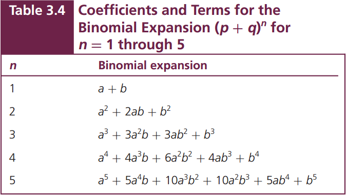
(p + q)5 = p5 + 5p4q + 10p3q2 + 10p2q3 + 5pq4 + q5
57
Each of the terms in the expansion provides the probability for one particular combination of traits in the children. The first term in the expansion (p5) equals the probability of having five children all with albinism, because p is the probability of albinism. The second term (5p4q) equals the probability of having four children with albinism and one with normal pigmentation, the third term (10p3q2) equals the probability of having three children with albinism and two with normal pigmentation, and so forth.
To obtain the probability of any combination of events, we insert the values of p and q; so the probability of having two out of five children with albinism is:

We could easily figure out the probability of any desired combination of albinism and pigmentation among five children by using the other terms in the expansion.
How did we expand the binomial in this example? In general, the expansion of any binomial (p + q)n consists of a series of n + 1 terms. In the preceding example, n = 5; so there are 5 + 1 = 6 terms: p5, 5p4q, 10p3q2, 10p2q3, 5pq4, and q5. To write out the terms, first figure out their exponents. The exponent of p in the first term always begins with the power to which the binomial is raised, or n. In our example, n equals 5, so our first term is p5. The exponent of p decreases by one in each successive term; so the exponent of p is 4 in the second term (p4), 3 in the third term (p3), and so forth. The exponent of q is 0 (no q) in the first term and increases by 1 in each successive term, increasing from 0 to 5 in our example.
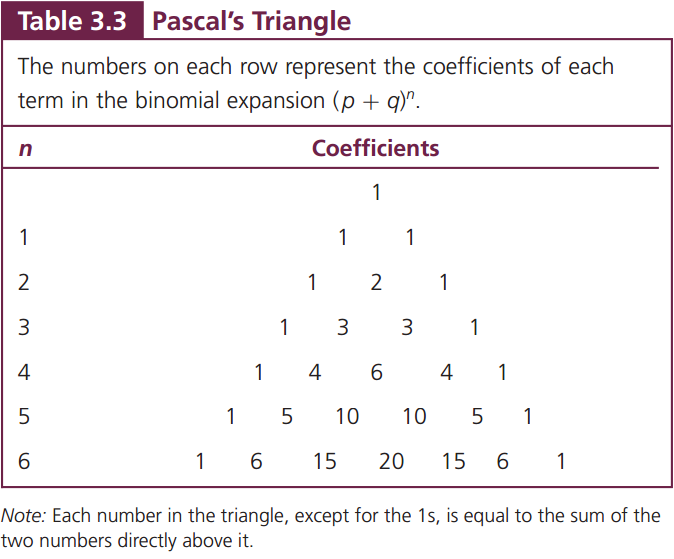
Next, determine the coefficient of each term. The coefficient of the first term is always 1; so, in our example, the first term is 1p5, or just p5. The coefficient of the second term is always the same as the power to which the binomial is raised; in our example, this coefficient is 5 and the term is 5p4q. For the coefficient of the third term, look back at the preceding term; multiply the coefficient of the preceding term (5 in our example) by the exponent of p in that term (4) and then divide by the number of that term (second term, or 2). So the coefficient of the third term in our example is (5 × 4)/2 =  = 10 and the term is 10p3q2. Follow this procedure for each successive term. The coefficients for the terms in the binomial expansion can also be determined from Pascal’s triangle (Table 3.3). The exponents and coefficients for each term in the first 5 binomial expansions are given in Table 3.4.
Another way to determine the probability of any particular combination of events is to use the following formula:

where P equals the overall probability of event X with probability p occurring s times and event Y with probability q occurring t times. For our albinism example, event X would be the occurrence of a child with albinism (
) and event Y would be the occurrence of a child with normal pigmentation (
); s would equal the number of children with albinism (2) and t would equal the number of children with normal pigmentation (3). The ! symbol stands for factorial, and it means the product of all the integers from n to 1. In this example, n = 5; so n! = 5 × 4 × 3 × 2 × 1. Applying this formula to obtain the probability of two out of five children having albinism, we obtain:
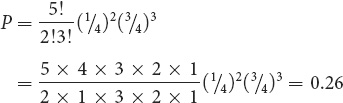
This value is the same as that obtained with the binomial expansion. ![]() TRY PROBLEMS 25, 26, AND 27
TRY PROBLEMS 25, 26, AND 27
The Testcross
A useful tool for analyzing genetic crosses is the testcross, in which one individual of unknown genotype is crossed with another individual with a homozygous recessive genotype for the trait in question. Figure 3.7 illustrates a testcross (in this case, it is also a backcross). A testcross tests, or reveals, the genotype of the first individual.
Suppose you were given a tall pea plant with no information about its parents. Because tallness is a dominant trait in peas, your plant could be either homozygous (TT) or heterozygous (Tt), but you would not know which. You could determine its genotype by performing a testcross. If the plant were homozygous (TT), a testcross would produce all tall progeny (TT × tt → all Tt); if the plant were heterozygous (Tt), half of the progeny would be tall and half would be short (Tt × tt →
Tt and
tt). When a testcross is performed, any recessive allele in the unknown genotype is expressed in the progeny, because it will be paired with a recessive allele from the homozygous recessive parent. ![]() TRY PROBLEMS 18 AND 21
TRY PROBLEMS 18 AND 21
58
CONCEPTS
The binomial expansion can be used to determine the probability of a particular set of events. A testcross is a cross between an individual with an unknown genotype and one with a homozygous recessive genotype. The outcome of the testcross can reveal the unknown genotype.
Genetic Symbols
As we have seen, genetic crosses are usually depicted with the use of symbols to designate the different alleles. The symbols used for alleles are usually determined by the community of geneticists who work on a particular organism and therefore there is no universal system for designating symbols. In plants, lowercase letters are often used to designate recessive alleles, and uppercase letters are for dominant alleles. Two or three letters may be used for a single allele: the recessive allele for heart-shaped leaves in cucumbers is designated hl, and the recessive allele for abnormal sperm-head shape in mice is designated azh.
In animals, the common allele for a character—called the wild type because it is the allele usually found in the wild—is often symbolized by one or more letters and a plus sign (+). The letter or letters chosen are usually based on the mutant (unusual) phenotype. For example, the recessive allele for yellow eyes in the Oriental fruit fly is represented by ye, whereas the allele for wild-type eye color is represented by ye+. At times, the letters for the wild-type allele are dropped and the allele is represented simply by a plus sign. Superscripts and subscripts are sometimes added to distinguish between genes: Lfr1 and Lfr2 represent dominant mutant alleles at different loci that produce lacerate leaf margins in opium poppies; ElR represents an allele in goats that restricts the length of the ears.
A slash may be used to distinguish alleles present in an individual genotype. For example, the genotype of a goat that is heterozygous for restricted ears might be written El+/ElR or simply +/ElR. If genotypes at more than one locus are presented together, a space separates the genotypes. For example, a goat heterozygous for a pair of alleles that produces restricted ears and heterozygous for another pair of alleles that produces goiter can be designated by El+/ElR G/g. Sometimes it is useful to designate the possibility of several genotypes. A line in a genotype, such as A_, indicates that any allele is possible. In this case, A_ might include both AA and Aa genotypes.
CONNECTING CONCEPTS: Ratios in Simple Crosses
Now that we have had some experience with genetic crosses, let’s review the ratios that appear in the progeny of simple crosses, in which a single locus is under consideration and one of the alleles is dominant over the other. Understanding these ratios and the parental genotypes that produce them will enable you to work simple genetic crosses quickly, without resorting to the Punnett square. Later, we will use these ratios to work more-complicated crosses that include several loci.
There are only three phenotypic ratios to understand (Table 3.5). The 3 : 1 ratio arises in a simple genetic cross when both of the parents are heterozygous for a dominant trait (Aa × Aa). The second phenotypic ratio is the 1 : 1 ratio which results from the mating of a heterozygous parent and a homozygous parent. The homozygous parent in this cross must carry two recessive alleles (Aa × aa) to obtain a 1 : 1 ratio, because a cross between a homozygous dominant parent and a heterozygous parent (AA × Aa) produces offspring displaying only the dominant trait.
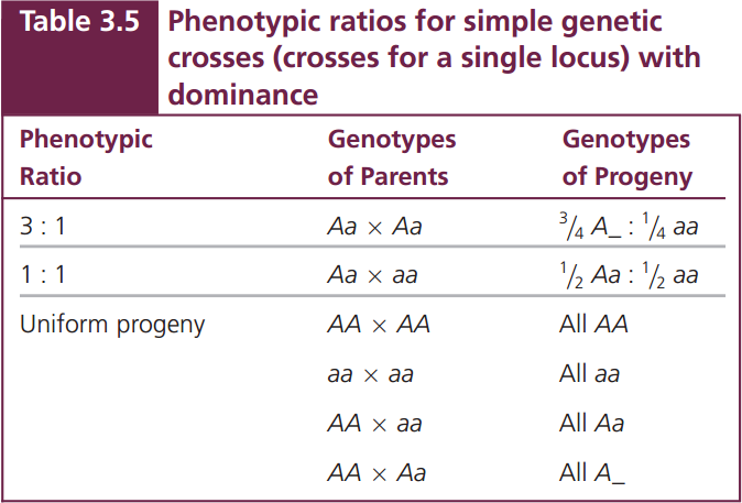
The third phenotypic ratio is not really a ratio: all the offspring have the same phenotype (uniform progeny). Several combinations of parents can produce this outcome (see Table 3.5). A cross between any two homozygous parents—either between two of the same homozygotes (AA × AA or aa × aa) or between two different homozygotes (AA × aa)—produces progeny all having the same phenotype. Progeny of a single phenotype also can result from a cross between a homozygous dominant parent and a heterozygote (AA × Aa).
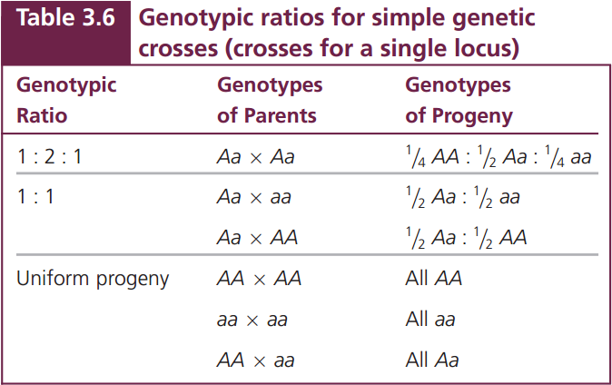
If we are interested in the ratios of genotypes instead of phenotypes, there are only three outcomes to remember (Table 3.6): the 1 : 2 : 1 ratio, produced by a cross between two heterozygotes; the 1 : 1 ratio, produced by a cross between a heterozygote and a homozygote; and the uniform progeny produced by a cross between two homozygotes. These simple phenotypic and genotypic ratios and the parental genotypes that produce them provide the key to understanding crosses for a single locus and, as you will see in the next section, for multiple loci.
59